The simulation of solute transport can be integrated in the groundwater flow simulation (see T03.Numerical groundwater modelling and optimization) using MT3DMS or MT3DMS-USGS. The implementation is based on FloPy (Bakker et al, 2016).
The solute transport tool in combination with groundwater flow simulation can be used for the optimization of MAR systems. Specifically, it can be applied to analyze water quality, geochemical processes, recovery efficiency and residence time in MAR schemes (Ringleb et al., 2016).
The spread of infiltrated treated wastewater in the aquifer at Shafdan, Israel was simulated using the groundwater flow model MODFLOW and the solute transport code MT3DMS and to evaluate different operation scenarios (Abbo and Gev, 2008). Both models also helped to improve the layout of groundwater monitoring wells and to determine the optimal hydraulic load, which is defined as the volume of water applied per time period, at a SAT site in China (Yin et al., 2006). The optimal infiltration pond operation and the transport of diazepem in an aquifer in Greece was analysed using MODFLOW and MT3DMS (Rahman, 2011). Wett, 2006 examined the clogging of a riverbank filtration system in Austria by simulating tracer tests. The hydraulic conductivity decreased by one order of magnitude through clogging resulting in a halving of infiltration rate during one year of operation. The behaviour of emerging organic contaminants during riverbank filtration was studied by Henzler, 2014. Ray and Prommer, 2006 studied the chemical transport of ethylene dibromide to extraction wells during a hypothetical emergency spill in Illinois, USA. They further investigated the transport of the herbicide atrazine throughout a flooding event during riverbank filtration.
The utilization of well-established simulation codes such as MODFLOW, and MT3DMS is favourable due to the existing wide application field and comprehensive documentation (Ringleb et al., 2016).
THEORETICAL BACKGROUND
The solute transport tool is mainly based on MT3DMS code, which is a modular three-dimensional transport model for multi-components, where MT3D stands for the Modular 3-Dimensional Transport model and MS means Multi-Species. It is capable to simulate advection, dispersion/diffusion and chemical reaction of contaminants in groundwater systems.
Advection means the transport of miscible contaminants at the same velocity as the groundwater. Dispersion in porous media describes the expansion of contaminants over a greater region than would be predicted solely from the groundwater velocity vectors. The chemical reaction is used for simulating general biological and geochemical reactions in the groundwater systems, which can be coped with equilibrium-controlled linear or non-linear sorption, nonequilibrium (rate-limited) sorption, and first-order reaction.
The transport of contaminants can be described with the following differential equation (Zheng and Wang, 1999):
\frac{\partial(\theta C^k)}{\partial t} = \frac{\partial}{\partial x_i}\Big(\theta D_{ij}\frac{\partial C^k}{\partial x_j} \Big) - \frac{\partial}{\partial x_i}(\theta v_i C^k) + q_s C^k_s + \Sigma R_nwhere
| C^k | the dissolved concentration of species k [ML-3] |
| \theta | the porosity of the subsurface medium [-] |
| t | time [T] |
| x_i | the distance along the respective Cartesian coordinate axis [L] |
| D_{ij} | the hydrodynamic dispersion coefficient tensor [L2T-1] |
| v_i | the seepage or linear pore water velocity [LT-1] |
| q_s | the volumetric flow rate per unit volume of aquifer representing fluid sources (positive) and sinks (negative) [T-1] |
| C^k_s | the concentration of the source or sink flux for species k [ML-3] |
| \Sigma R_n | the chemical reaction term [ML-3T-1] |
The three-dimensional advection-dispersion-reaction equation in the MT3DMS code can be solved by the standard finite difference method; the particle-tracking-based Eulerian-Lagrangian methods; and the higher-order finite-volume TVD method.
SUPPORTED MT3DMS PACKAGES
| BTN | Basic transport package | BTN is necessary for all solute transport simulations, which provides all the basic information for the solute transport model (e.g. boundary and initial conditions) |
| ADV | Avection Package | ADV is an optional package in the simulation. It is chosen when the concentration changes due to advection. |
| DSP | Dispersion Package | DSP is an optional package in the simulation. It is required when the concentration changes owing to dispersion. |
| SSM | Source Sink Package | SSM is an optional package in the simulation. It is used when the concentration changes because of sink/source mixing. |
| GCG | Matrix Solver Package | GCG is used for solving the matrix equations resulting from the implicit solution of the transport equations. |
Further packages, such as the Reaction (RCT) Package, will be integrated in the future.
MODEL SETUP
The transport function is active when the ‘Enabled’ box is marked. Two versions of MT3D (MT3DMS and MT3D-USGS) can be selected to simulate solute transport on the platform.
The changes will not be automatically saved in the system. Please click the "save" button when you want to keep the changes in each dialogue box.
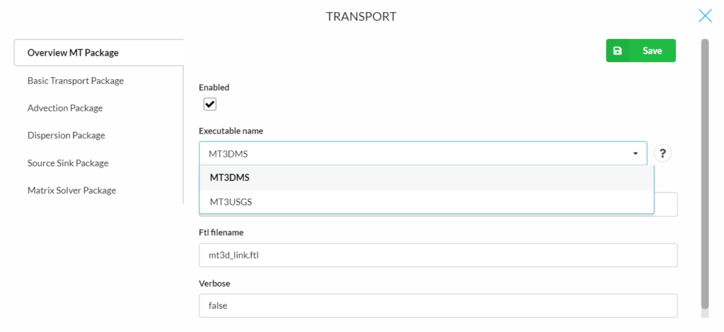
A more specific explanation for the variables can be found in the question mark after each variable.
Basic Transport Package
The following parameters are required for the Basic Transport Package:
Basic parameters
- Total species (Ncomp): The total number of chemical species in the simulation (Defaut is 1).
- Mobile species (Mcomp): The total number of ‘mobile’ species. mcomp must be equal or less than ncomp (Defaut is 1).
- Porosity (Prsity): The effective porosity of the porous medium in a single porosity system, or the mobile porosity in a dual-porosity medium (Defaut is 0.3).
- Concentration boundary indicator (Icbund): The Icbund specifies the boundary condition type for solute species (shared by all species).
- If icbund = 0, the cell is an inactive concentration cell;
- If icbund < 0, the cell is a constant-concentration cell;
- if icbund > 0, the cell is an active concentration cell where the concentration value will be calculated.(Defaut value is 1)
- Starting concentration (Sconc): The Sconc defines the starting concentration for the first species (Defaut is 0).
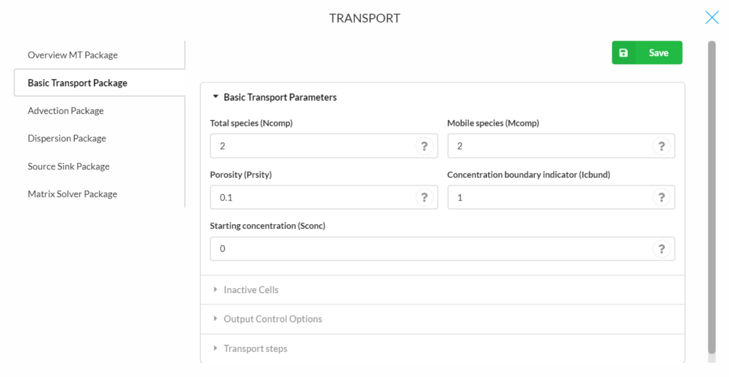
The platform only works for one species at the moment. Also, icbund and sconc can only be defined as a single value for the whole model domain.
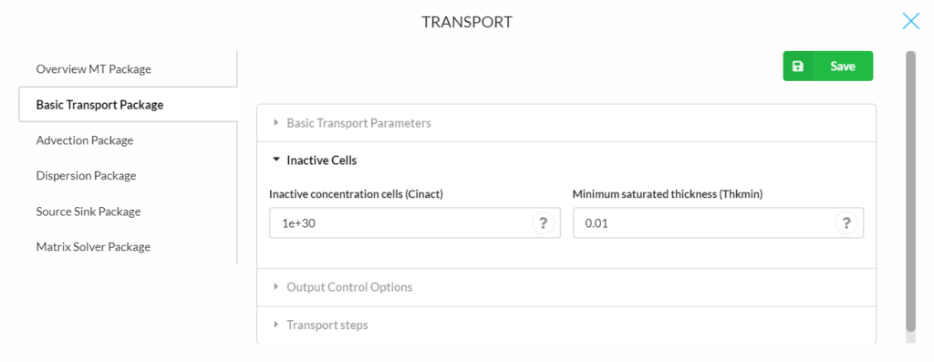
Inactive cells
- Inactive concentration cells (Clinact): The value for indicating an inactive concentration cell (Default is 1e+30).
- Minimum saturated thickness (Thkmin): The minimum saturated thickness in a cell, expressed as the decimal fraction of its thickness, below which the cell is considered inactive (Default is 0.01, which equals 1% of the model thickness).
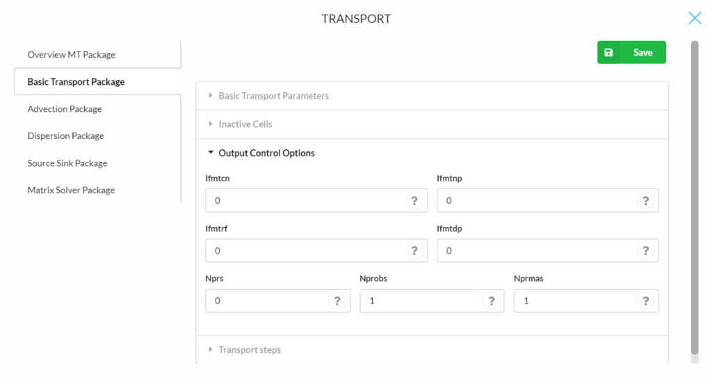
Output Control Options
- Ifmtcn: A flag/format code indicating how the calculated concentration should be printed to the standard output text file. Format codes for printing are listed in Table 3 of the MT3DMS manual (Zheng and Wang, 1999, Default is 0).
- If ifmtcn > 0 printing is in wrap form;
- ifmtcn < 0 printing is in strip form;
- if ifmtcn = 0 concentrations are not printed.
- Ifmtnp: A flag/format code indicating how the number of particles should be printed to the standard output text file. The convention is the same as for ifmtcn (Default is 0).
- Ifmtrf: A flag/format code indicating how the calculated retardation factor should be printed to the standard output text file. The convention is the same as for ifmtcn (Default is 0).
- A flag/format code indicating how the distance-weighted dispersion coefficient should be printed to the standard output text file. The convention is the same as for ifmtcn (Default is 0).
- Nprs: A flag indicating (i) the frequency of the output and (ii) whether the output frequency is specified in terms of total elapsed simulation time or the transport step number.
- If nprs > 0 results will be saved at the times as specified in timprs;
- if nprs = 0, results will not be saved except at the end of simulation (Default);
- if nprs < 0, simulation results will be saved whenever the number of transport steps is an even multiple of nprs. .
- Nprobs: An integer indicating how frequently the concentration at the specified observation points should be saved (Default is 1).
- Nprmas: An integer indicating how frequently the mass budget information should be saved (Default is 1).
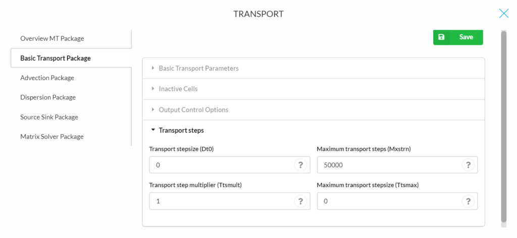
Transport steps
- Transport stepsize (Dt0): The user-specified initial transport step size within each time-step of the flow solution (Default is 0).
- Maximum transport steps (Mxstrn): The maximum number of transport steps allowed within one time step of the flow solution (Default is 50 000).
- Transport step multiplier (Ttsmult): The multiplier for successive transport steps within a flow time-step if the GCG solver is used and the solution option for the advection term is the standard finite-difference method (Default is 1.0).
- Maximum transport stepsize (Ttsmax): The maximum transport step size allowed when transport step size multiplier TTSMULT > 1.0 (Default is 0).
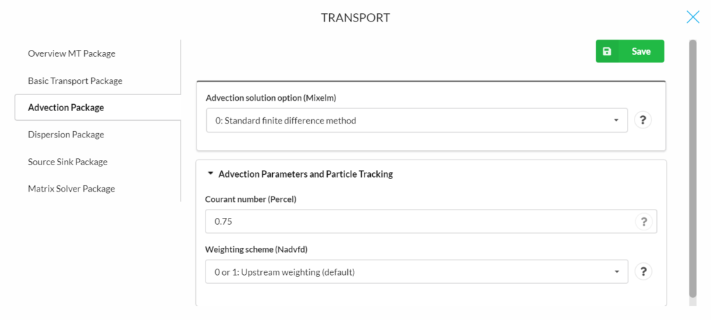
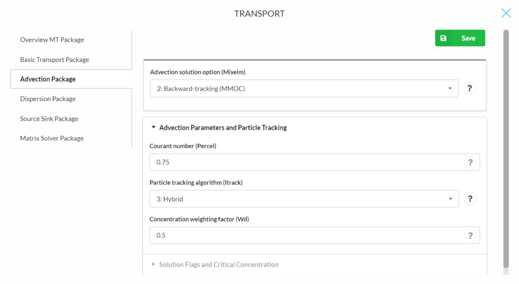
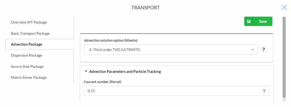
Advection Package
- Mixelm = 0 is the standard finite-difference method with upstream or central-in-space weighting;
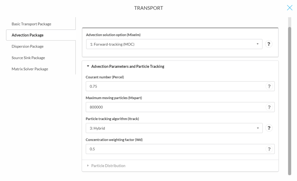
- Mixelm = 1 is the forward-tracking method of characteristics (MOC);
- Mixelm = 2 is the backward-tracking modified method of characteristics (MMOC);
- Mixelm = 3 is the hybrid method of characteristics (HMOC) with MOC or MMOC automatically and dynamically selected; and
- Mixelm = -1, the third-order TVD (Total variation diminishing) scheme (ULTIMATE).
The various solution schemes are explained in the following in detail.
Mixelm = 0 is the standard finite-difference method with upstream or central-in-space weighting, depending on the value of NADVFD. The following parameters are for determining advection and particle tracking :
- Courant number (Percel): PERCEL is the Courant number (i.e., the number of cells, or a fraction of a cell) advection will be allowed in any direction in one transport step. For implicit finite-difference or particle-tracking-based schemes, there is no limit on PERCEL, but for accuracy reasons, it is generally not set much greater than one. Note, however, that the PERCEL limit is checked over the entire model grid. Thus, even if PERCEL > 1, advection may not be more than one cell’s length at most model locations. For the explicit finite-difference or the third-order TVD scheme, PERCEL is also a stability constraint which must not exceed one and will be automatically reset to one if a value greater than one is specified.
- Weighting scheme (Nadvfd):
- Nadvfd = 0 or 1, upstream weighting (Default);
- Nadvfd = 2, central-in-space weighting.
Mixelm = 1 is the forward-tracking method of characteristics (MOC). The following parameters are for determining advection and particle tracking:
- Courant number (Percel), explanation see above.
- Maximum moving particles (Mxpart)
- Particle tracking algorithm (Itrack): ITRACK is a flag indicating which particle-tracking algorithm is selected for the Eulerian-Lagrangian methods.
- ITRACK = 1, the first-order Euler algorithm is used.
- ITRACK = 2, the fourth-order Runge-Kutta algorithm is used; this option is computationally demanding and may be needed only when PERCEL is set greater than one.
- ITRACK = 3, the hybrid first- and fourth-order algorithm is used;
- the Runge-Kutta algorithm (ITRACK=2) is used in sink/source cells and the cells next to sinks/sources while the Euler algorithm (ITRACK=1) is used elsewhere.
- Concentration weighting factor (Wd): is a concentration weighting factor between 0.5 and 1. It is used for operator splitting in the particle- tracking-based methods. The value of 0.5 is generally adequate. The value of WD may be adjusted to achieve better mass balance. Generally, it can be increased toward 1.0 as advection becomes more dominant (Default is 0.5).
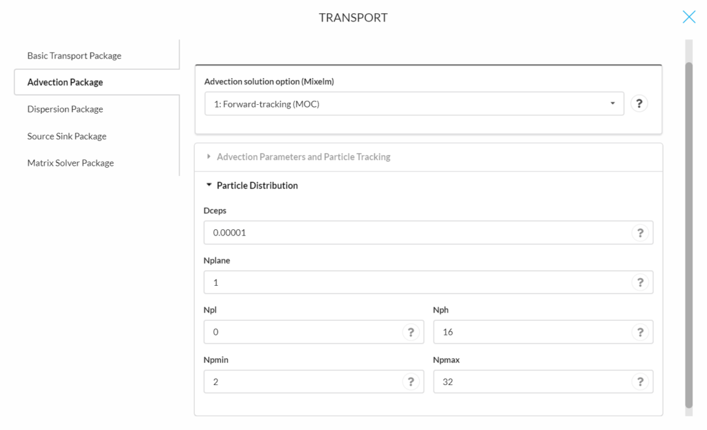
The following parameters are for determining particle distribution:
- Dceps: is a small Relative Cell Concentration Gradient below which advective transport is considered.
- Nplane: NPLANE is a flag indicating whether the random or fixed pattern is selected for initial placement of moving particles.
- If NPLANE = 0, the random pattern is selected for initial placement. Particles are distributed randomly in both the horizontal and vertical directions by calling a random number generator. This option is usually preferred and leads to smaller mass balance discrepancy in nonuniform or diverging/converging flow fields.
- If NPLANE > 0, the fixed pattern is selected for initial placement. The value of NPLANE serves as the number of vertical ‘planes’ on which initial particles are placed within each cell block. The fixed pattern may work better than the random pattern only in relatively uniform flow fields. For two-dimensional simulations in plan view, set NPLANE = 1. For cross sectional or three-dimensional simulations, NPLANE = 2 is normally adequate. Increase NPLANE if more resolution in the vertical direction is desired.
- Npl: is the number of initial particles per cell to be placed at cells where the Relative Cell Concentration Gradient is less than or equal to DCEPS. Generally, NPL can be set to zero since advection is considered insignificant when the Relative Cell Concentration Gradient is less than or equal to DCEPS. Setting NPL equal to NPH causes a uniform number of particles to be placed in every cell over the entire grid (i.e., the uniform approach).
- Nph: is the number of initial particles per cell to be placed at cells where the Relative Cell Concentration Gradient is greater than DCEPS. The selection of NPH depends on the nature of the flow field and also the computer memory limitation. Generally, a smaller number should be used in relatively uniform flow fields and a larger number should be used in relatively nonuniform flow fields. However, values exceeding 16 in two-dimensional simulation or 32 in three- dimensional simulation are rarely necessary. If the random pattern is chosen, NPH particles are randomly distributed within the cell block. If the fixed pattern is chosen, NPH is divided by NPLANE to yield the number of particles to be placed per vertical plane.
- Npmin: is the minimum number of particles allowed per cell. If the number of particles in a cell at the end of a transport step is fewer than NPMIN, new particles are inserted into that cell to maintain a sufficient number of particles. NPMIN can be set to zero in relatively uniform flow fields and to a number greater than zero in diverging/converging flow fields. Generally, a value between zero and four is adequate.
- Npmax: is the maximum number of particles allowed per cell. If the number of particles in a cell exceeds NPMAX, all particles are removed from that cell and replaced by a new set of particles equal to NPH to maintain mass balance. Generally, NPMAX can be set to approximately two times of NPH.
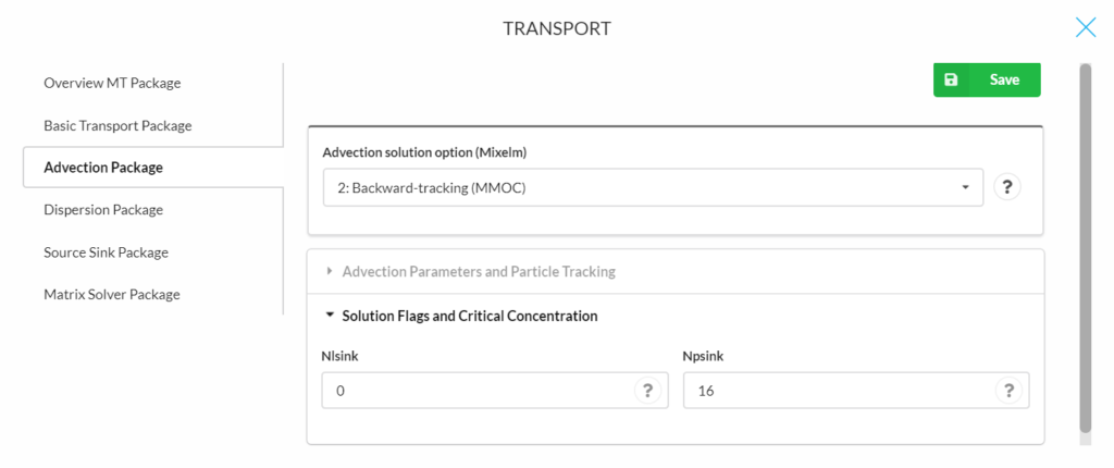
Mixelm = 2 is the backward-tracking modified method of characteristics (MMOC). The following parameters are for determining advection and particle tracking (for explanations of the parameters see other solution methods above):
- Conrant number (Percel)
- Particle tracking algorithm (Itrack)
- Concentration weighting factor (Wd)
The following parameters are for solution flags and critical concentration:
- Nlsink: is a flag indicating whether the random or fixed pattern is selected for initial placement of particles to approximate sink cells in the MMOC scheme. The convention is the same as that for NPLANE. It is generally adequate to set NLSINK equivalent to NPLANE.
- Npsink: is the number of particles used to approximate sink cells in the MMOC scheme. The convention is the same as that for NPH. It is generally adequate to set NPSINK equivalent to NPH.
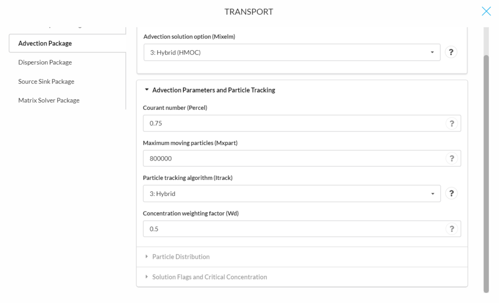
Mixelm = 3 is the hybrid method of characteristics (HMOC) with MOC or MMOC automatically and dynamically selected. The following parameters are for determining advection and particle tracking (for explanations of the parameters see other solution methods above):
- Conrant number (Percel)
- Maximum moving particles (Mxpart)
- Particle tracking algorithm (Itrack)
- Concentration weighting factor (Wd)
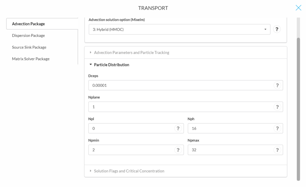
The following parameters are for determining particle distribution (for explanations of the parameters see other solution methods above):
- Dceps
- Nplane
- Npl
- Nph
- Npmin
- Npmax
The following parameters are for solution flags and critical concentration (for explanations of the parameters see other solution methods above):
- Nlsink
- Npsink

Mixelm = -1, the third-order TVD scheme (ULTIMATE). This scheme is applied for solving the advection term that is mass conservative and minimizes numerical dispersion and artificial oscillation. The following parameters are for determining advection and particle tracking:
- Conrant number (Percel)
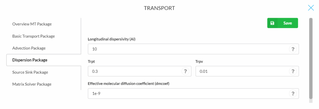
Dispersion Package
- Longitudinal dispersivity (Al): is the longitudinal dispersivity, for every cell of the model grid (unit, L, Default is 0.01).
- Trpt: is the ratio of the horizontal transverse dispersivity to the longitudinal dispersivity. Field studies suggest that TRPT is generally not greater than 0.1 (Default is 0.1).
- Trpv: is the ratio of the vertical transverse dispersivity to the longitudinal dispersivity. Field studies suggest that TRPT is generally not greater than 0.01(Default is 0.01).
- Effective molecular diffusion coefficient (dmcoef): is the effective molecular diffusion coefficient (unit, L2T-1). Set DMCOEF = 0 if the effect of molecular diffusion is considered unimportant (Default is 1.e-9).
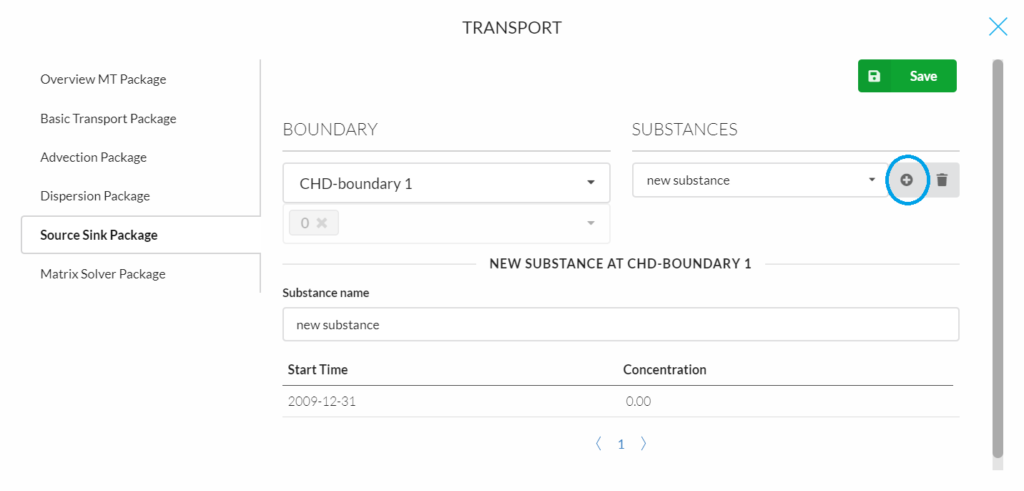
Source Sink Package
- Determine which boundary would be the source/ sink in the simulation.
- Click the “plus mark” (in the blue round rectangular) to add a new substance.
- Define the substance name, start time and concentration in the upcoming windows.
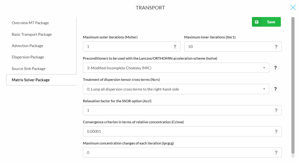
Matrix Solver Package
- Maximum outer iterations (Mxiter): is the maximum number of outer iterations; it should be set to an integer greater than one only when a nonlinear sorption isotherm is included in simulation (Default is 1).
- Maximum inner iterations (Lter1): is the maximum number of inner iterations; a value of 30-50 should be adequate for most problems (Default is 50).
- Preconditioners to be used with the Lanczos/ORTHOMIN acceleration scheme, an algorithm for solving a system of linear equations (Brezinski and Redivo‐Zaglia, 1998, Isolve):
- = 1, Jacobi (a method of solving a matrix equation on a matrix that has no zeros along its main diagonal (Bronshtein et al. 2007));
- = 2, SSOR (Symmetric Successive Over Relaxation);
- = 3, Modified Incomplete Cholesky (MIC) (MIC usually converges faster, but it needs significantly more memory, Default).
- Treatment of dispersion tensor cross terms (Ncrs):
- = 0, lump all dispersion cross terms to the right-hand-side (approximate but highly efficient, Default);
- = 1, include full dispersion tensor (memory intensive).
- Relaxation factor for the SSOR option (Accl): is the relaxation factor for the SSOR option; a value of 1.0 is generally adequate (Default is 1).
- Convergence criterion in terms of relative concentration (Cclose): is the convergence criterion in terms of relative concentration; a real value between 10-4 and 10-6 is generally adequate (Default is 1.E-5).
- Maximum concentration changes of each iteration (iprgcg): IPRGCG is the interval for printing the maximum concentration changes of each iteration. Set IPRGCG to zero as default for printing at the end of each stress period (Default is 0)
 .
.
RESULTS
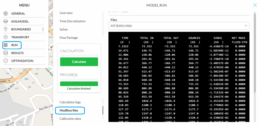
The model output such as the mass balance and model list file can be viewed on the “run” section.
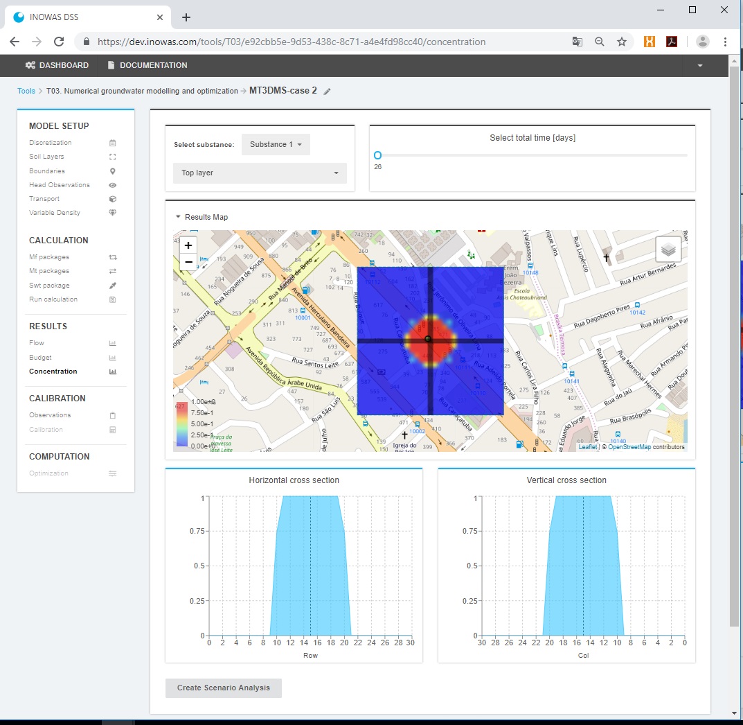
Concentration
An overview of solute concentration in the selected layer and row can be displayed on the platform (same as the visualization of groundwater head). For that the substance, layer and stress periods can be selected.
External Links
For more information on the individual packages and program functionalities, see the Flopy mt3dms online guide and MT3DMS Documentation and User’s Guide.
References
- Abbo, H. and Gev, I. (2008). Numerical model as a predictive analysis tool for rehabilitation and conservation of the Israeli Coastal Aquifer: example of the SHAFDAN Sewage Reclamation project. Desalination, 226(1-3):47–55, doi:10.1016/j.desal.2007.01.233.
- Bakker, M., Post, V., Langevin, C.D., Hughes, J.D., White, J.T., Starn, J.J., Fienen, M.N., 2016. Scripting MODFLOW Model Development Using Python and FloPy. Groundwater 54, 733–739. doi:10.1111/gwat.12413
- Bedekar, V., Morway, E.D., Langevin, C.D., and Tonkin, M., 2016, MT3D-USGS version 1: A U.S. Geological Survey release of MT3DMS updated with new and expanded transport capabilities for use with MODFLOW: U.S. Geological Survey Techniques and Methods 6-A53, 69 p., http://dx.doi.org/10.3133/tm6A53
- Brezinski, C.; Redivo‐Zaglia, M. (1998). In Numerical Algorithms 17 (1/2), pp. 67–103. DOI: 10.1023/A:1012085428800.
-
Bronshtein, Ilja N.; Muehlig, Heiner; Musiol, Gerhard; Semendyayev, Konstantin A. (2007): Handbook of Mathematics. 5th Ed. Berlin, Heidelberg: Springer-Verlag Berlin Heidelberg. Available online at https://ebookcentral.proquest.com/lib/subhh/detail.action?docID=645334.
- Henzler, A. F., Greskowiak, J., and Massmann, G. (2014). Modeling the fate of organic micropollutants during river bank filtration (Berlin, Germany). Journal of Contaminant Hydrology, 156:78–92, doi:10.1016/j.jconhyd.2013.10.005.
- Rahman, M. A. (2011). Decision Support for Managed Aquifer Recharge (MAR) Project Planning to Mitigate Water Scarcity based on Non-conventional Water Resources. Dissertation, Georg-August-Universität zu Göttingen.
- Ray, C. and Prommer, H. (2006). Clogging-Induced Flow and Chemical Transport Simulation in Riverbank Filtration Systems. In Hubbs, S., editor, Riverbank Filtration Hydrology, volume 60 of Nato Science Series: IV: Earth and Environmental Sciences, pages 155–177. Springer Netherlands.
-
Ringleb, Jana; Sallwey, Jana; Stefan, Catalin (2016): Assessment of Managed Aquifer Recharge through Modeling—A Review. In Water 8 (12), p. 579. DOI: 10.3390/w8120579.
- Wett, B. (2006). Monitoring Clogging of a RBF-System at the river Enns, Austria. In Hubbs, S., editor, Riverbank Filtration Hydrology, volume 60 of Nato Science Series: IV: Earth and Environmental
Sciences, p. 155–177. Springer Netherlands. -
Yin, H. and Xu, Z. and Li, H. and Li, S. (2006): Numerical modeling of wastewater transport and degradation in soil aquifer. Journal of Hydrodynamics, B, p. 597–605.
- Zheng, C. and Wang, P. P. (1999) MT3DMS: A Modular Three-dimensional Multi species Transport Model for Simulation of Advection, Dispersion, and Chemical Reactions of Contaminants in Ground Water Systems. https://hydro.geo.ua.edu/mt3d/mt3dmanual.pdf
- Zheng, Chunmiao, 2010, MT3DMS v5.3 Supplemental User’s Guide, Technical Report to the U.S. Army Engineer Research and Development Center, Department of Geological Sciences, University of Alabama, 51 p. https://hydro.geo.ua.edu/mt3d/mt3dms_v5_supplemental.pdf