Variable-density flow can be added to the numerical groundwater flow and transport simulation using SEAWAT. The implementation is based on FloPy (Bakker et al, 2016). A requirement is that a groundwater flow model was setup (see T03.Numerical groundwater modelling and optimization) and solute transport is active (see T03b. Solute transport (MT3DMS)).
The tool can be e.g. used to assess saltwater intrusion in coastal aquifers and the impact of Managed Aquifer Recharge (MAR) schemes to mitigate saltwater intrusion.
Many case studies have been conducted to assess the influence of MAR on saltwater intrusion. A focus has been on the impact of MAR on the extent of seawater intrusion, the recovery efficiency and the planning of new MAR facilities or the optimization of existing ones. Pauw et al., 2015 examined the impact of artificial recharge and drainage system on a freshwater lense in a reclaimed tidal flat plain in the Netherlands using the density-driven numerical flow and transport model SEAWAT. They concluded that the freshwater lense increased by MAR and more water can be extracted. Russo et al., 2015 combined GIS and modeling to identify suitable MAR sites and to assess the hydrologic impact and operating scenarios to reduce sea water intrusion in a coastal aquifer in California, USA. Glaß, 2019 examined the influence of viscosity on seasonal travel time during MAR operation in Berlin, Germany using SEAWAT.
THEORETICAL BACKGROUND
The following paragraph is taken from Glaß, 2019:
“The following solute transport equation is adapted to simulate heat transport using SEAWAT (Langevin et al., 2008):
\left(1+\frac{1-n_{e}}{n_{e}}\frac{\rho_{soil}c_{s}}{\rho_{F}c_{F}}\right)\frac{\delta(n_{e}T)}{\delta t}=\nabla\left[n_{e}\left(\frac{\lambda_{b}}{n_{e}\rho_{F}c_{F}}+\alpha\frac{q}{n_{e}}\right)\nabla T\right]-\nabla(qT)-q\text{´}_{s}T_{s}where n_{e} is effective porosity [-], \rho_{soil} is the density of the soil [ML -3], c_{S} is the specific heat of the solid [L 2T -2 °C -1], \alpha is the dispersivity tensor [L], q{´}_{s} a source or sink [L -1] and T_{s} is the sink/source temperature [°C]. T is temperature [°C], t is time [T], \lambda_{b} describes the bulk thermal conductivity of the rock-fluid matrix [ML 3T -2°C -1] , \rho_{b} and \rho_{F} are the density of the rock-fluid matrix and fluid [ML -3], c_{b} and c_{F} are the specific heat of the rock-fluid matrix and the fluid [L 2T -2 °C -1] and q is the Darcy velocity or specific discharge [LT -1].
To represent thermal equilibrium between the fluid and solid, heat conduction and the specific heat flux, the following specific relations are required (Vandenbohede and Van Houtte, 2012):
The retardation coefficient is the consequence of the equilibration of temperature between the fluid and the solid and causes the temperature front to move slower than the average flow velocity (Vandenbohede and Van Houtte, 2012). For that, a linear sorption isotherm is utilized in the chemical reaction package of MT3DMS (Vandenbohede and Van Houtte, 2012). The thermal distribution coefficient K_{DT} [L 3M -1] is defined as:
K_{DT}=\frac{c_{S}}{\rho_{F}c_{F}}From which the thermal retardation R [-] can be calculated:
R=1+\frac{\rho_{b}}{n_{e}}K_{DT}The solute transport process of molecular diffusion is mathematically similar to thermal conduction. Hence, the thermal diffusion coefficient is used for the temperature species which is also called the bulk thermal diffusivity D_{T} [L 2T -1]:
D_{T}=\frac{\lambda_{b}}{n_{e}\rho_{F}c_{F}}\;\;\;\textrm{where}\:\;\lambda_{b}=n_{e}\lambda_{F}+(1-n_{e})\lambda_{S}where λ_{F} is the thermal conductivity of the fluid, λ_{S} of the solid phase and λ_{b} the bulk thermal conductivity [ML 3T -2°C -1].
The viscosity \mu [ML -1T -1] is considered to be solely a function of temperature (Langevin et al., 2008).”
FloPy is used to create, run and post-process the SEAWAT models.
MODEL SETUP
In the model setup section, variable-density flow can be enabled if solute transport is active. This requirement is necessary as S EAWAT uses some solute transport parameters for the simulation. In addition, the change of viscosity can be included into the simulations. In that way also temperature can be simulated.
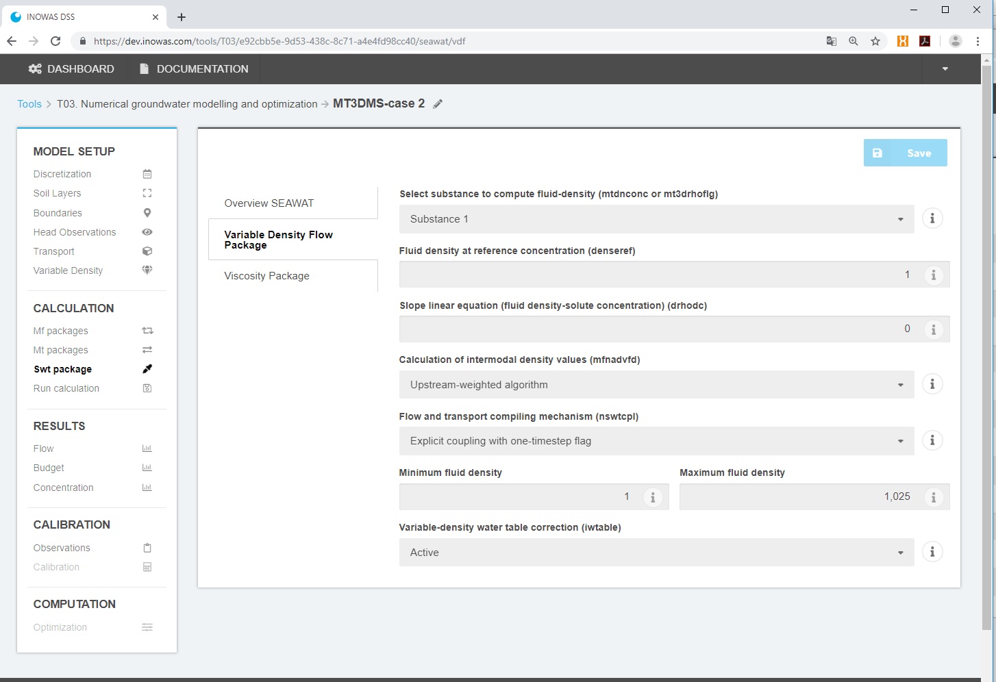
Variable-Density Flow Package
- Select substance to compute fluid-density (mtdnconc or mt3drhoflg)
- Fluid density at reference concentration (denseref)
- Slope linear equation (fluid density-solute concentration) (drhodc)
- Calculation of intermodal density values (mfnadvfd)
- Upstream-weighted algorithm
- Central-in-space algorithm
- Flow and transport compiling mechanism (nswtcpl)
- Explicit coupling with one-timestep flag
- Non-linear coupling iterations
- Number of iterations
- Convergence criterion
- Limited recalculation of flow solution
- Minimum fluid density
- Maximum fluid density
- Variable-density water table correction (iwtable)
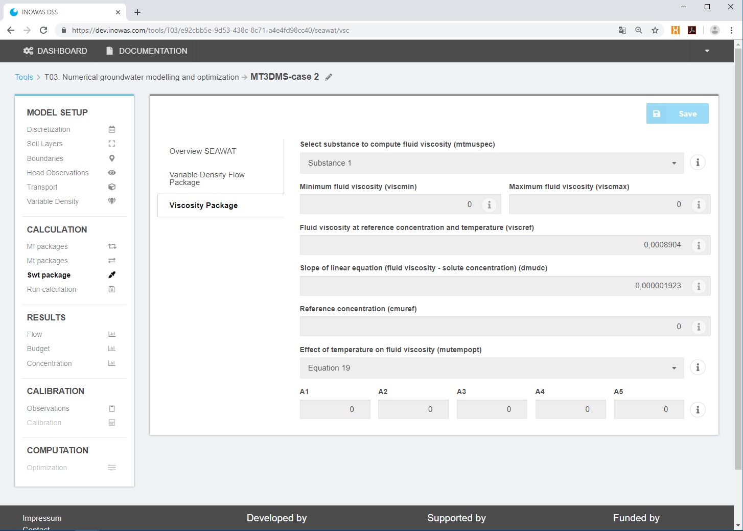
Viscosity Package
- Select substance to compute fluid viscosity (mtmuspec)
- Minimum fluid viscosity (viscmin)
- Maximum fluid viscosity (viscmax)
- Fluid viscosity at reference concentration and temperature (viscref)
- Slope of linear equation (fluid viscosity – solute concentration) (dmudc)
- Reference concentration (cmuref)
- Effect of temperature on fluid viscosity (mutempopt)
- None
- Equation 18 (Langevin et al., 2008): \mu_{T}(T)=A_{1}A_{2}^{(\frac{A_{3}}{T+A_{4}})}
The following relation is often stated in the literature (Voss, 1984):
\mu(T)=293.4*10^{-7}*10^{\left(\frac{248.37}{T+133.15}\right)} - Equation 19 (Langevin et al., 2008): \mu_{T}(T)=A_{1}\left[A_{2}+A_{3}(T+A_{4})\right]^{A_{5}}
- Equation 20 (Langevin et al., 2008): \mu_{T}(T)=A_{1}T^{A_{2}}
 RESULTS
The resulting concentration can be displayed as described in the Results Section for solute transport (see T03b. Solute transport (MT3DMS)).
External Links
For more information on the individual packages and program functionalities, see the Flopy seawat online guide and SEAWAT Documentation and User’s Guide.
References
- Bakker, M., Post, V., Langevin, C.D., Hughes, J.D., White, J.T., Starn, J.J., Fienen, M.N., 2016. Scripting MODFLOW Model Development Using Python and FloPy. Groundwater 54, 733–739. doi:10.1111/gwat.12413
- Glaß, J., 2019. New advances in the assessment of managed aquifer recharge through modelling. Technische Universität Dresden, Dresden, Germany.
- Langevin, C. D., Thorne, D. T., Drausman, A. M., Sukop, M. C. & Guo, W. SEAWAT Version 4: A Computer Program for Simulation of Multi-Species Solute and Heat Transport. 39 p. (2008).
- Pauw, P.S., van Baaren, E.S., Visser, M., de Louw, P.G.B., Essink, G.H.P.O., 2015. Increasing a freshwater lens below a creek ridge using a controlled artificial recharge and drainage system: a case study in the Netherlands. Hydrogeology Journal 23, 1415–1430. doi:10.1007/s10040-015-1264-
- Ringleb, Jana; Sallwey, Jana; Stefan, Catalin (2016): Assessment of Managed Aquifer Recharge through Modeling—A Review. In Water 8 (12), p. 579. DOI: 10.3390/w8120579.
- Russo, T.A., Fisher, A.T., Lockwood, B.S., 2015. Assessment of Managed Aquifer Recharge Site Suitability Using a GIS and Modeling. Groundwater 53, 389–400. doi:10.1111/gwat.12213
- Vandenbohede, A., Van Houtte, E., 2012. Heat transport and temperature distribution during managed artificial recharge with surface ponds. Journal of Hydrology 472–473, 77–89. https://doi.org/10.1016/j.jhydrol.2012.09.028
-
Voss, C.I., 1984. SUTRA, Saturated-Unsaturated TRAnsport: A Finite-Element Simulation Model for Saturated-Unsaturated Fluid-Density-Dependent Groundwater Flow with Energy Transport or Chemically Reactive Single-Species Solute Transport (No. 84–4369), Water Resources Investigations, Report. US Geological Survey.