This tool can be used for setting up a new numerical groundwater flow and solute transport model.
The most widely applied numerical model for MAR assessment is MODFLOW which is a numerical groundwater flow model developed by the USGS (Harbaugh, 2005; Ringleb et al., 2016). The INOWAS tool helps to setup a new MODFLOW model for a study area in order to better understand the local groundwater flow system or as a basis for further scenario analysis (see T07. MODFLOW model scenario manager). The tool is based on MODFLOW-2005 (Harbaugh, 2005) and FloPy (Bakker et al., 2016) and enables the user to create, write and read input and output files as well as calculate models. In addition, solute transport using MT3DMS can be added to the groundwater flow model (see T03b. Solute transport (MT3DMS)) as well as variable-density flow (see T03c. variable-density flow (SEAWAT)). The INOWAS platform furthermore provides optimization algorithms to find the best location for an ASR well using a calibrated groundwater flow and solute transport model.
THEORETICAL BACKGROUND
Flow model (MODFLOW)
MODFLOW-2005 is based on the Darcy equation (Darcy, 1856):
Where
| k | = hydraulic conductivity [L/T] |
| | = fluid velocity [L/T] |
| | = change of hydraulic head [L] |
| = length of the flow domain [L] | |
| A | = cross-sectional area of flow [L²] |
| Q | = discharge [L³/T] |
- Discretization
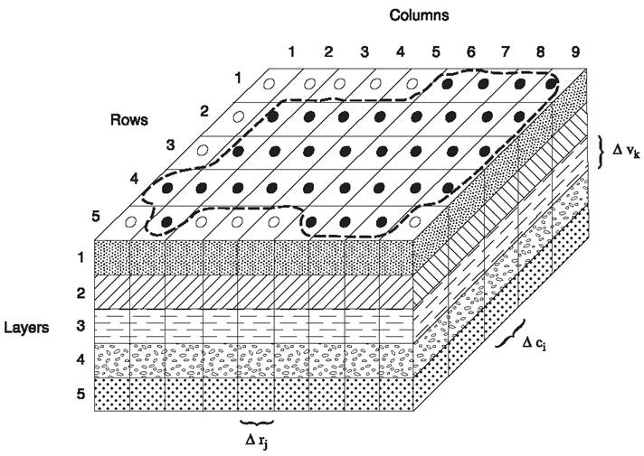
MODFLOW is a modular finite-difference model solving the groundwater flow equation in three dimensions and it is used to simulate the flow of groundwater through aquifers. The flow domain is discretized by a grid containing cells. For each cell the head is calculated in the center of the cell (node). Only active cells (Figure, filled points) are regarded in the calculation. Inactive cells (Figure, circle) are ignored.
- Boundary conditions
Boundary conditions are necessary to define how the user-specified model interacts with the surrounding flow system. In a natural system boundaries can be physical (e.g. sharp changes in hydraulic conductivity) or hydraulic (e.g. groundwater divides, streamlines). These boundaries need to be approximated in the model. In MODFLOW constant-head and no-flow cells are used to represent conditions along various hydrologic boundaries inside the grid. No allocation is needed to indicate no flow at the edge of the model area as MODFLOW does not compute inter-cell flow through the outside edges of the grid (including bottom and top). Table 1 gives an overview of the three available main boundary conditions including examples when those boundary conditions are generally used:
Table 1. Main types of boundary conditions
| Type | Example | |||
| H=constant | 1st type | Dirichlet | specified head | aquifer border, river, lake |
| Q=constant (Q=0) | 2nd type | Neumann | specified flux | aquifer border (Q=0), barrier, recharge, pumping wells |
| Q=f(H) | 3rd type | Cauchy | flux as function of potential (mixed condition) | river with additional resistance as a colmation layer |
- Hydraulic parameters
Hydraulic parameters which describe the rock framework are hydraulic conductivity, transmissivity and specific storage (yield). Those parameters influence the modeling results the most together with boundary conditions.
- Steady state vs. transient simulations
In steady-state simulations the storage term in the groundwater flow equation becomes zero. The head is a function of the location and ignores time changes. A steady-state problem only requires a single solution of simultaneous equations. In comparison to that, a transient simulation solves multiple solutions for multiple time steps. In transient simulations the head is a function of location and time. Therefore, the initial condition of the modeling area (e.g. distribution of hydraulic head at starting time) needs to be specified. For steady-state simulation there is no direct requirement for initial head as the time derivate is removed from the flow equation. However, often initial head is specified as an initial estimate to start the iterative process.
- Conceptual model
The conceptual model is capturing important features and processes of the geologic, hydrologic and geomechanical environment as an approximation of the reality and is the basis for the numerical model. Developing a good conceptual model requires compiling detailed information on geological formation, groundwater flow direction, recharge, surface water, hydraulic parameters, extraction or injection from wells, and the groundwater quality (Hesch and Chmakov, 2011). Next to parameter uncertainties especially conceptualization uncertainties are constraining the reliability and robustness of a numerical model and therefore the conceptual framework needs to be designed carefully.
- Calibration, validation and sensitivity analysis
The calibration comprises the adjustment of model parameters, boundary conditions and model concept until the simulated values match field observations. Methods incorporate manual (try&error) and automatic calibration. For validation, model results are compared to results from field observation for a different time frame than calibration. Typical questions such as “Are the results plausible?”, “Is the model oversimplified?” or “Is the model sensitive to changes of specific parameters?” need to be answered at that step. Sensitivity analysis helps to identify parameters and observations which have the most influence on modeling results. A calibrated model is necessary for reliable results and prognosis.
- Scenario Analysis (see T07. MODFLOW model scenario manager)
With the help of the calibrated model scenarios analyses can be conducted to incoporate future development into the modeling study. The analysis can include assessment of the impact of land use change as well as climate change on the groundwater. The implementation of MAR schemes in the study area including their impact on groundwater levels, on saltwater intrusion or their interference with other groundwater users can be assessed by building different scenarios.
MODEL SETUP
The following section describes in a stepwise manner how to setup, run and calibrate a new groundwater flow model by using this tool.Optionally, solute transport and density-driven flow can be added.
The changes will not be automatically saved in the system. Please click the "save" button when you want to keep the changes in each dialogue box.
The coordinate system on the INOWAS platform is WGS84 (EPSG identifier: 4326). Please be aware that all spatial data that you upload is referenced to that coordinate system.
General
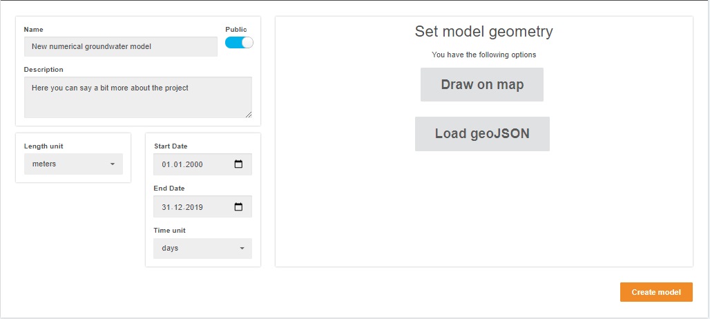
A new MODFLOW model can be created which includes the assignment of a Model Name. A description can be added. The time and length units need to be chosen from a dropdown list. At the moment, only meters and days are supported. Be aware that the units selection will be valid throughout the whole model setup and all parameters need to be inserted using the same units.
- Time units: seconds, minutes, hours, days, months, years
- Length units: centimeters, meters, feet
- Grid Resolution: Type in the number of columns and the number of rows.The grid is displayed in the Area window.
- Time resolution: type in the start and end date of your model. This can be still changed and new stress periods can be added later.
- Model area: can be defined by drawing a polygone on the map. With the help of the GIS-tools the user can draw, edit and save the model area polygone. Alternatively, a json file can be uploaded in the dashboard via the import function. Be aware, that the json needs to be in the exact format as descripted in the model import section.
- Spatial discretization: The cell numbers along rows and columns can be selected.
- Time discretization: The start and end date can be defined.
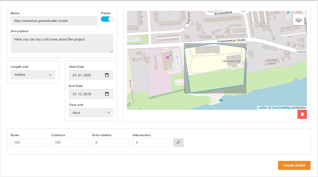
- Grid rotation: The grid can be roated by a specified rotation angle.
- Intersection: The intersection is automatically calculated.
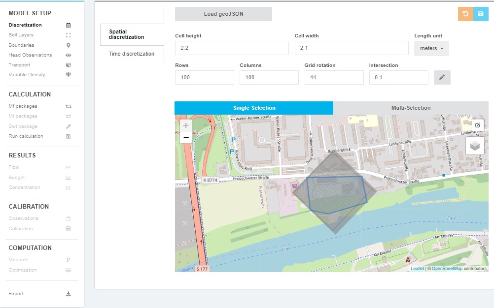
Discretization
Spatial discretization
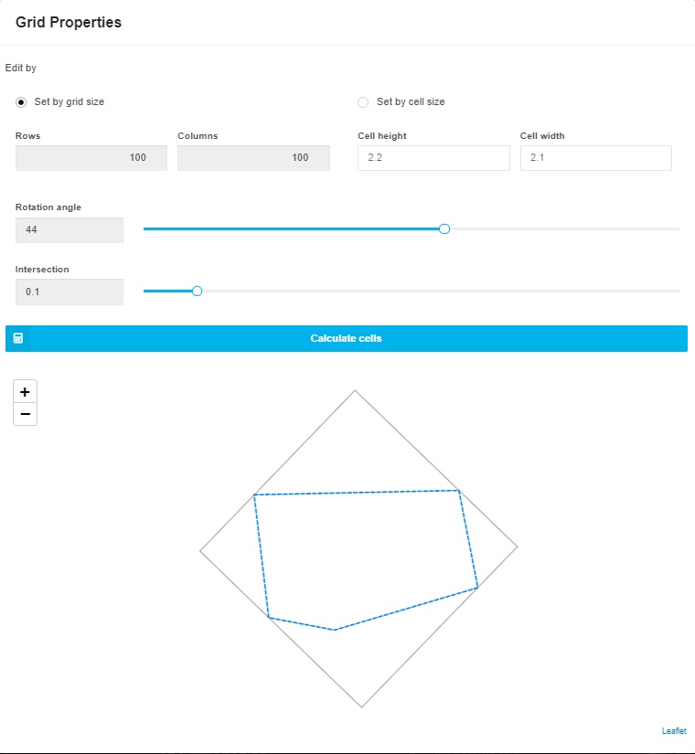
After creating the model and assigning the general model parameters, the spatial discretization can be viewed and the model area as well as the cell size, the number of rows and columns and the specified grid rotation can be edited.
Time discretization
In this window, the overall time frame of the model (including Start and End date) as well as the number and type of Stress Periods can be edited. Stress Periods are time intervals during which boundary conditions are constant. For each Stress Period the following parameters need to be defined:
- Starting Time: the starting date of the stress period in format dd:mm:yyyy hh:minmin.
- Ending Time: the ending point of the stress period is automatically transferred from the starting point of the next stress period or the end date of the model.
- Number of Time Steps (nstp): number of time steps within the current Stress Period.
- Time Step Multiplier (tsmult) to calculate the length of the Time Steps within the current Stress Period.
- State of the Stress Period: steady state or transient.
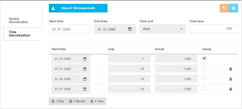
The table can be edited: new Stress Periods can be added by using the “+1 day“,”+1 month” or “+1 year” button. The Start Date can be manually edited. The End Date is automatically assigned from the Start Date of the consequent Stress period or the End Date of the whole simulation for the last Stress Period. Existing Stress Periods can be deleted by using the “Delete” button.
It is also possible to import stress periods using the CSV Upload.
Soil Layers
In the soil model dialogue box new model layers and zones can be added or model layer properties can be assigned. As default, one model layer exists called “0:Top Layer”.
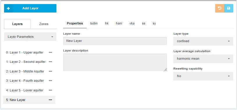
Create new model layer
A new layer can be added by using the “Add layer” button. The following general layer properties can be assigned or edited:
- Layer name: name of the layer
- Layer description: description of the layer
- Layer type: two options are available. Confined if the conductance terms for cell-to-cell flow are calculated at the beginning of the simulation and remain constant or convertible if the conductance term gets updated at each iteration step with the help of the saturated thickness.
- Layer average calculation (Interblock transmissivity): three options are available. Describes the method that is used to calculate the interblock transmissivity. Harmonc mean which is most appropriate for aquifers with abrupt transmissivity boundaries or confined aquifers with uniform hydraulic conductivity. Logarithmic mean which is most appropriate for confined aquifers with gradually varying transmissivities or arithmetic mean of saturated thickness and logarithmic-mean hydraulic conductivity which is most appropriate for unconfined aquifers with gradually varying transmissivities.
- Wetting Capability: two options are available. Active indicates that cells which become dry during a simulation can be rewetted. Inactive indicates that cells can not be rewetted once dry.
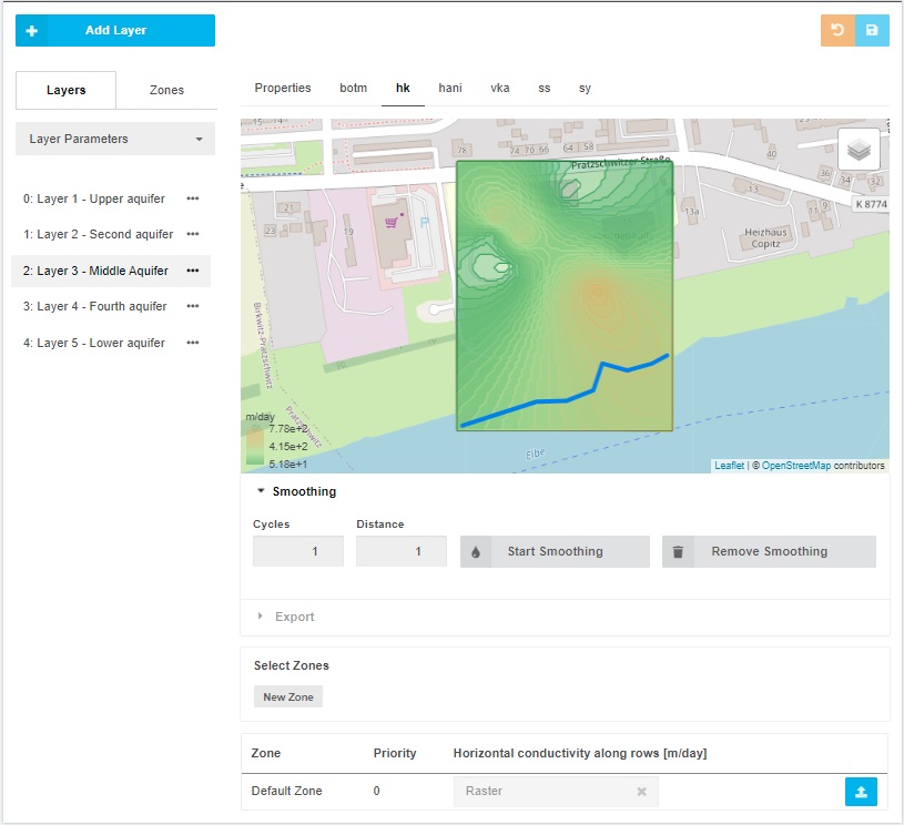
Model Layer Properties
Once a model layer is created, layer properties can be assigned. There are different options to assign layer properties:
- Set constant values for all grid cells
- Upload properties from existing Raster file
- Apply zones to layers and define parameter values for applied zones (see the description for zones further below)
- Smooth the assigned values by cycles or distance
The following soil layer properties can be defined (“Layer parameters” in drop down menue):
- Top elevation: surface elevation of the model layer [L].
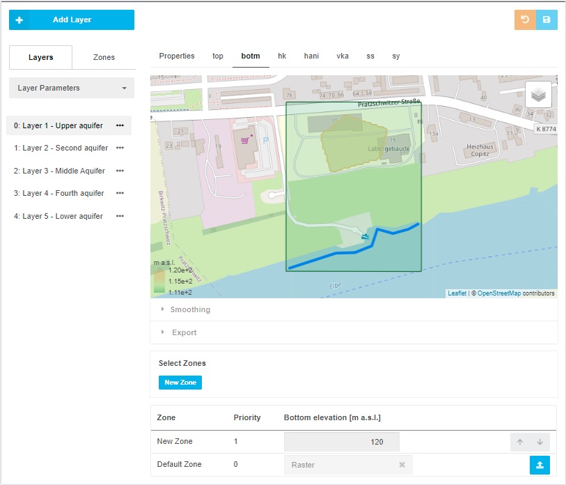
- Bottom elevation (botm): bottom surface of the model layer [L].
- hk: hydraulic conductivity along the x-direction also referred to as horizontal hydraulic conductivity [L/T].
- hani: ratio between the hydraulic conductivity along the y-direction and x-direction [L/T].
- vka: hydraulic conductivity along the z-direction also referred to as vertical hydraulic conductivity [L/T].
- Ss: specific storage [1/L]. It is only read for a transient simulation.
- Sy: specific yield. It is only read for a transient simulation and if the layer is convertible.
In addition, basic layer properties can be assigned by choosing “Basic Layer Properties” in the drop down menue:
- IBOUND: active cells of the model layer. The default is the model area defined in the spatial discretization section.
- STRT: starting head [L] of the model layer. The default is the top elevation of the model.
The assigned soil parameter raster can be exported for top and bottom elevation (top, botm) and the horizontal and vertical conductivities (hk, vka) as well as IBOUND and STRT.
Zones
Zones can be used to vary a parameter within a layer and the model boundaries. They can be created by using the “Zones” tab. A pop-up window opens, where the new zone can be defined by name and shape.
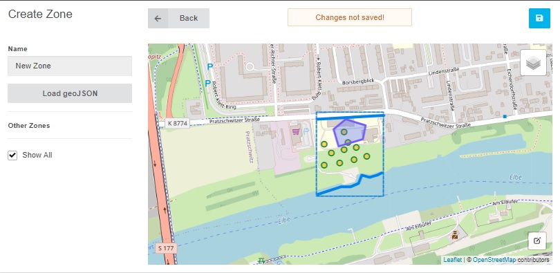
These zones can be applied to every layer and every layer parameter seperately. To activate a zone for a specific parameter, go to the layer property and Select the desired zone. A constant value can be defined for the zone in the table (see figure below).
Flow boundary conditions
The geometry of a boundary can be added by uploading a json file or defining the geometry by hand. Depending on the boundary, the geometry equals a point (e.g. WEL), line (e.g. CHD) or area (e.g. RCH) which can be defined using the GIS tools of the INOWAS platform or by including the coordinates of the geometrical points that define the geometry in the json file (an example file can be downloaded in the Import section after a boundary has been created manually).
Time series data for a boundary can be either included in the json file, uploaded by CSV or assigned manually. Be aware that the decimal separator in the CSV file must be point. The column separator can be either comma or semicolon. The number of data points in the CSV file must be equal to the number of stress periods in the model.
1) Specified head boundaries
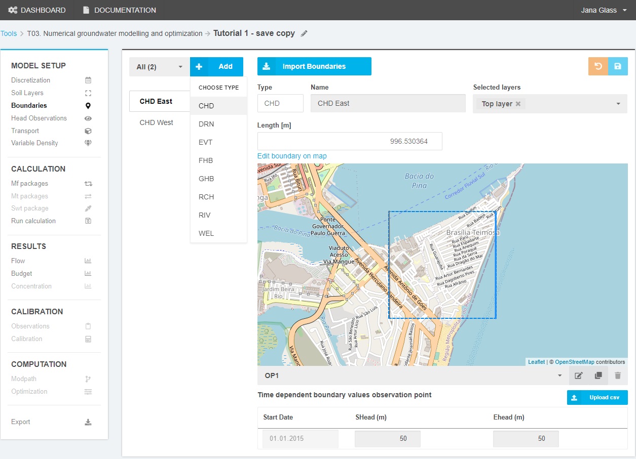
Time-Variant Specified Head (CHD)
The CHD-Package is used to simulate specified head boundaries that can change within or between stress periods.
- Name: define name of the specified head boundary.
- CHD Line: Draw a Polyline directly on the map. The tool then automatically assigns the intersecting cells to the constant head boundary. The affected cells can be viewed by clicking on “Edit boundary on map”. It is also possible to assign specific cells to the boundary by clicking on the map or to delete specific cells from the boundary condition.
- Layer: Defines the layer to which the constant head boundary is applied. Select the layer from the list.
For each time period the following parameters need to be defined:
- Starting Specified Head (SHead): define the head [L] at the beginning of each time period defined.
- Ending Specified Head (EHead): define the head [L] at the end of each time period defined.
- Define the Start Date of various specified heads. The End Date is automatically assigned from the Start Date of the consequent specified head or the End date of the model.
Flow and Head Boundary Package (FHB)
The FHB Package is used for specified head and specified flow cells, whose properties can vary within a stress period.
- FHB name: Define a refernce name for the FHB boundary
- FHB line: Draw a Polyline directly on the map. The tool then automatically assigns the intersecting cells to the constant head boundary. The affected cells can be viewed by clicking on “Edit boundary on map”. It is also possible to assign specific cells to the boundary by clicking on the map or to delete specific cells from the boundary condition.
- Layer: Defines the layer to which the flow and head boundary is applied. Select the layer from the list.
For each time period the following parameters need to be defined:
- Date: Is the date on which values of specified head or flow will be read.
- Head: defines the head [L] at each specified date.
- Flow: defines the flow at each specified date.
Choose whether to assign specified flow or specified head by ticking the respective box in the table head.
2) Specified flux boundaries:
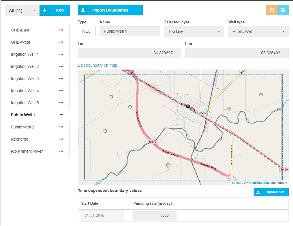
Wells (WEL)
The Well-Package allows to simulate abstraction of groundwater or recharge to an aquifer to an individual cell. Therefore, a specified positive flux (recharge) or negative flux (abstraction) is defined. The following parameters need to be assigned:
- Well name: Define a reference name for the well.
- Well location: Draw a point on the map. The tool then automatically assigns the intersecting cells to the constant head boundary. The affected cells can be viewed by clicking on “Edit boundary on map”. It is also possible to assign specific cells to the boundary by clicking on the map or to delete specific cells from the boundary condition.
- Layer: is the layer number where the well is screened and recharges or abstracts water.
For each time period the following parameters need to be defined:
- Pumping rate: is the volumetric recharge rate [L³/T] for each time period. Positive indicates recharge and negative indicates discharge/ pumping.
- For each Pumping rate the Start Date needs to be defined. The End Date is automatically assigned from the Start Date of the consequent Pumping rate or the End date of the model.
Recharge (RCH)
The Recharge-Package is used to simulate a specified flux distributed over the top of the model. The user-defined recharge rates are multiplied by the horizontal areas of the cells to which they are applied to calculate the volumetric recharge flux.
- Name: Name of the recharge area.
- Recharge Area: the Model Area to which recharge is applied. A Polygone can be drawn on the map. The affected cells can be viewed by clicking on “Edit boundary on map”. It is also possible to assign specific cells to the boundary by clicking on the map or to delete specific cells from the boundary condition.
- Recharge Layer: is the layer to which recharge is applied. This property can be changed in the “Mf packages” section. Default is the top layer.
For each time period the following parameters need to be defined:
- Recharge Rate: is the recharge flux [L/T] for each time period.
- For each Recharge rate the Start Date needs to be defined. The End Date is automatically assigned from the Start Date of the consequent Recharge rate or the End date of the model.
3) Head-dependent flux boundaries
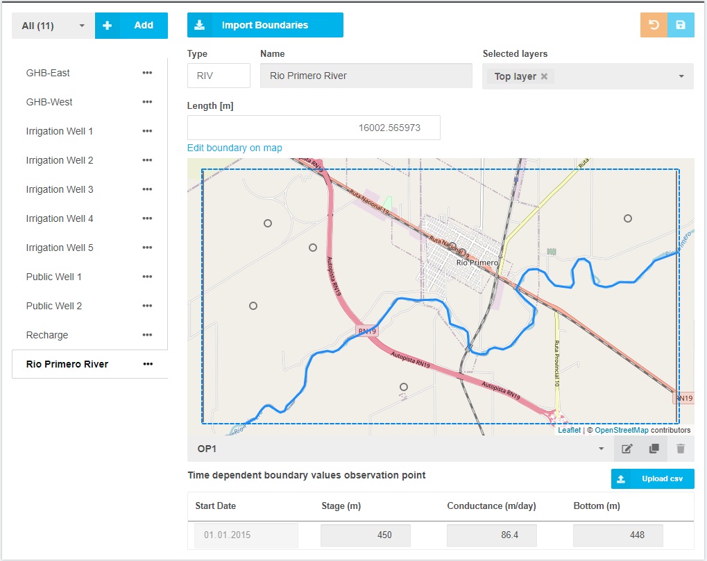
Rivers (RIV)
- Name: define name of the river.
- River Course: To assign the river course, the user can draw a Polyline directly on the map. The tool then automatically assigns the intersecting cells to the river boundary. The affected cells can be viewed by clicking on “Edit boundary on map”. It is also possible to assign specific cells to the boundary by clicking on the map or to delete specific cells from the boundary condition.
- Layer: Number of layer to which the river is in contact. This value is automatically calculated for each cell dependent on the location of the River bottom.
For each time period the following parameters need to be defined:
- River Stage: is the head [L] in the river for each time period.
- Conductance: Hydraulic conductance [L²/T] of the riverbed sediments for each time period.
- River Bottom: is the elevation of the bottom of the riverbed [L] for each time period.
- For each River stage the Start Date needs to be defined. The End Date is automatically assigned from the Start Date of the consequent River stage or the End date of the model.
General Head (GHB)
The General Head Boundary Package is used to simulate head-dependent flux boundaries where the flux is proportional to the difference in head.
- Name: define name of the general head boundary.
- GHB Line: To create a GHB boundary in the model area, the user can draw a Polyline directly on the map. The tool then automatically assigns the intersecting cells to the general head boundary. The affected cells can be viewed by clicking on “Edit boundary on map”. It is also possible to assign specific cells to the boundary by clicking on the map or to delete specific cells from the boundary condition.
- Layer: Defines the layer to which the general head boundary is applied.
For each time period the following parameters need to be defined:
- Head: defines the head [L] at the boundary for each time period.
- Conductance: Hydraulic conductance [L²/T] between the external source and each grid cell for each time period.
- For each General head the Start Date needs to be defined. The End Date is automatically assigned from the Start Date of the consequent General head or the End date of the model.
Evapotranspiration (EVT)
The Evapotranspiration Package is used to simulate a head-dependent flux out of the model distributed on top of the model [L/T]. Those rates are multiplied by the horizontal area of the cells to receive volumetric flux rates.
- Name: Name of the evapotranspiration area.
- Evapotranspiration Option Code (NEVTOP): determines the cell within a column for which evapotranspiration will be calculated:
- 1- EVT is calculated only for cells in the top grid layer
- 2- the cell for each vertical column is specified by user in variable IEVT
- 3- EVT is applied to the highest active cell in each vertical column.
- Evapotranspiration Area: the area of the model domain where evapotranspiration is assigned to.
For each stress period the following parameters need to be defined:
- Start Date of various evapotranspiration time periods.
- Maximum Evapotranspiration Flux (EVTR): defines the maximum evpotranspiration flux as volumetric flow rate per unit area [L/T].
- Elevation of Evapotranspiration Surface (SURF): equals the elevation of the Evapotranspiration Surface.
- Extinction depth (EXDP): is the extinction depth and refers to distance from SURF not elevation.
Drain (DRN)
The Drain Package is used to simulate head-dependent flux boundaries. If the head in the cell falls below a certain treshold, the flux from the drain to the model cell drops to zero. For each drain segment, a new boundary needs to be assigned.
- Name: Name of the Drain Segment.
- Drain Segment: Add Line-Shapefile or create a Line on the map to assign the drain segment.
- Layer number: Number of model layer to which the drain is in contact.
For each stress period the hydraulic conductance (C) of the drain bed sediments within each cell needs to be defined which can be calculated as follows:
with C is hydraulic Conductance [L²/T], KD is hydraulic conductivity [L/T] of the drain bed sediments, L is the length of the cell [L], WD is the width of the drain [L] and TD is the thickness of the drain bed sediments [L].
The parameters are linearly interpolated along the drain segment.
- Start Date of various drain segment time periods.
- Stage: drain elevation [L] at the upstream cell of the drain segment.
- Conductance [L²/T]: is the hydraulic conductance of the drain bed sediments.
Head observations
Head observations are useful for model calibration and can be included in the Head observations menue. The observed heads can be integrated manually or uploaded by CSV. It is also planned to integrate the possibility to include head observation directly from the INOWAS monitoring tool (“T10 Real-time monitoring”).

Calculation
In this step all relevant MODFLOW parameters for calculating the model can be set.
 The parameters for the following Packages can be edited:
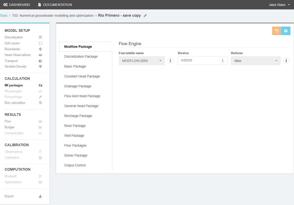
MODFLOW Package
- Executable name: at the moment, only MODFLOW-2005 as executable can be chosen.
Discretization Package
Gives an overview of the spatial and time discretization as well as the layer parameters that were assigned in the “Discretization” and “Soil Layers” sections.
Basic Package
The following parameters can be viewed:
- Boundary variable (ibound): defines whether a cell is active (ibound=1) which means that hydraulic head will be calculated at each iteration or inactive (ibound=0) where the groundwater flow equation is not solved. Furthermore, an active specified head cell (ibound=-1) is a cell where the hydraulic head is specified and will not vary throughout the simulation.
- Starting Head (STRT or Initial Head): is the initial starting head at the beginning of a simulation [L] and needs to be defined for all simulations including steady-state for all layers.
Flow Package
The flow package can be chosen in that section. At the moment, the current packages are implemented:
- Layer-Property Flow package (LPF)
- Block-Centered Flow package (BCF6)
Rewetting parameters
These parameters are only relevant, if wetting was activated for any layer.
-
- Rewetting factor (WETFCT): this factor is used to calculate an initially established head in a cell when it is converted from dry to wet.Default value is 0.1.
- Iteration interval (IWETIT): iteration interval for attempting to wet cells and applies to outer iterations. Default value is 1.
- Rewetting equation (IHDWET): a flag which determines the equation used to define the initial head at cells that become wet. If IHDWET=0, the following equation is used:
where
is the head in the neighboring cell that causes the dry cell to become wet. If IHDWET=1 (which is the default), the following equation is used:
.
- Wetting treshold (WETDRY): is a combination of the wetting threshold and a flag to indicate which neighboring cells can cause a dry cell to become wet. It is only read if the Wetting Capability is active for the layer and the Layer Type is convertible. Three options are available: if WETDRY<0 only the cell below can cause a dry cell to become wet, if WETDRY>0 a cell below the dry cell and the four horizontally adjacent cells can cause a cell to become wet and if WETDRY=0 the dry cell cannot be wetted. The absolute value of WETDRY is the wetting threshold.
Solver Package
At the moment, the Preconditioned Conjugate- GradientPackage (PCG) or the Direct Solver Package (DE4) can be chosen.
PCG Solver Parameters
For all solver parameters default values are already defined according to Table 3. The user can change the default parameters to its need. For an explanation of the parameters see the Online Guide to MODFLOW-2005 or Harbaugh, 2005.
Table 3. Default PCG Solver parameters.
| Parameter (MODFLOW labeling) | Default |
| Outer iterations (MXITER) | 50 |
| Inner iterations (ITER1) | 30 |
| Matrix conditioning method (NPCOND) | Modified Incomplete Cholesky |
| Head change criterion for convergence (HCLOSE) | 0.00001 |
| Residual criterion for convergence (RCLOSE) | 0.00001 |
| Relaxation Parameter (RELAX) | 1.0 |
| nbpol | 0 |
| Printout interval for PCG (IPRPCG)0 | 0 |
| Print options (mutpcg) | 3 |
| Steady-state damping Factor (DAMP) | 1.0 |
| Transient damping factor (dampt) | 1 |
| ihcofadd | 0 |
DE4 Package
For all solver parameters default values are already defined according to Table 4.
Table 4. Default DE4 Solver parameters.
| Outer iterations (itmx) | 50 |
| Maximum number of upper equations (mxup) | 0 |
| Maximum number of lower equations (mxlow) | 0 |
| Maximum bandwidth (mxbw) | 0 |
| Frequency of change (ifreq) | 0 |
| 0 | |
| Head change multiplier (accl) | 1 |
| 0.00001 | |
| Interval for time step printing (iprd4) | 1 |
Output Control
In the output control, parameters can be assignet that control:
- Format for printing head (ihedfm)
- Format for printing drawdown (iddnfm)
- Format saving head (chedfm)
- Format saving drawdown (cddnfm)
- Format saving ibound (cboufm)
Furthermore, it can be selected, whether the Head, drawdown and/or budget should be saved for the various Stress periods.
Boundary Packages
Package-specific parameters can be edited if the corresponding boundary is active in the model.
Run calculation
Once all the required simulation parameters are defined the simulation can be run using the Calculate button in the “Run Calculation” section. The calculation progress is shown. If the simulation terminated successfully, there will be a report from MODFLOW, showing the various calculated stress periods and whether the simulation terminated normal.
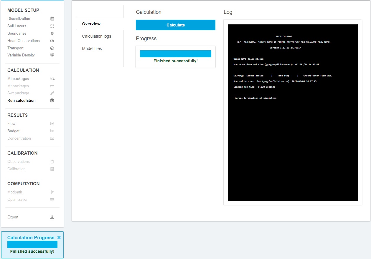
If the simulation terminated not normally or did not converge, the model input needs to be revised. As there are many reasons for model nonconvergence, see the “Guide on model convergence” to receive some tips to solve the issue.
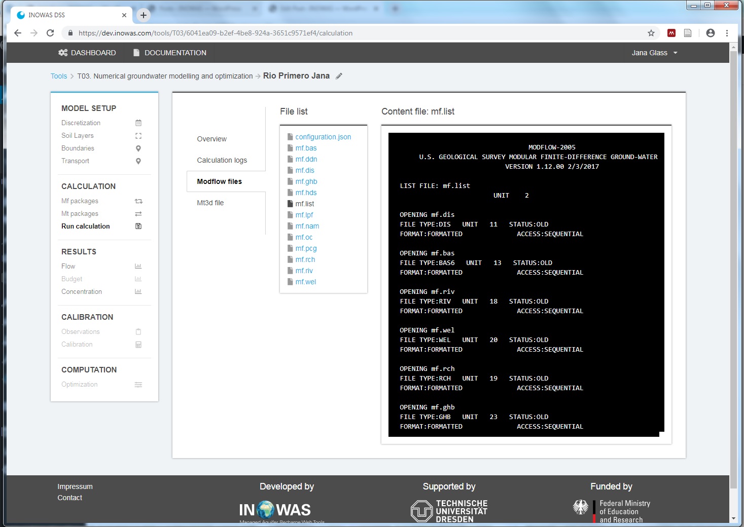
MODFLOW files
The various MODFLOW files can be viewed in that section.
The MODFLOW List File contains several useful information about the simulation run (for more information see Harbaugh, 2005). The file includes information about the time and spatial descritization of the model, the boundary conditions chosen, the solver parameters, the number of iterations for each time steps and the volumetric budget for each time step as well as the cumulative volumes.
It also includes information of the model run and should be consulted if a simulation did not terminate normal.
RESULTS
In this section of the tool simulation results can be viewed. Next to groundwater heads, the drawdown can be displayed and analysed.
Flow
Cross Section
By default, the groundwater heads within the model area are displayed for the first time step of the simulation period. The layer and whether groundwater heads or drawdown is displayed can be selected from a dropdown list. The time step can be chosen. A cross section of groundwater heads or drawdown can be displayed by selecting a specific row and column.
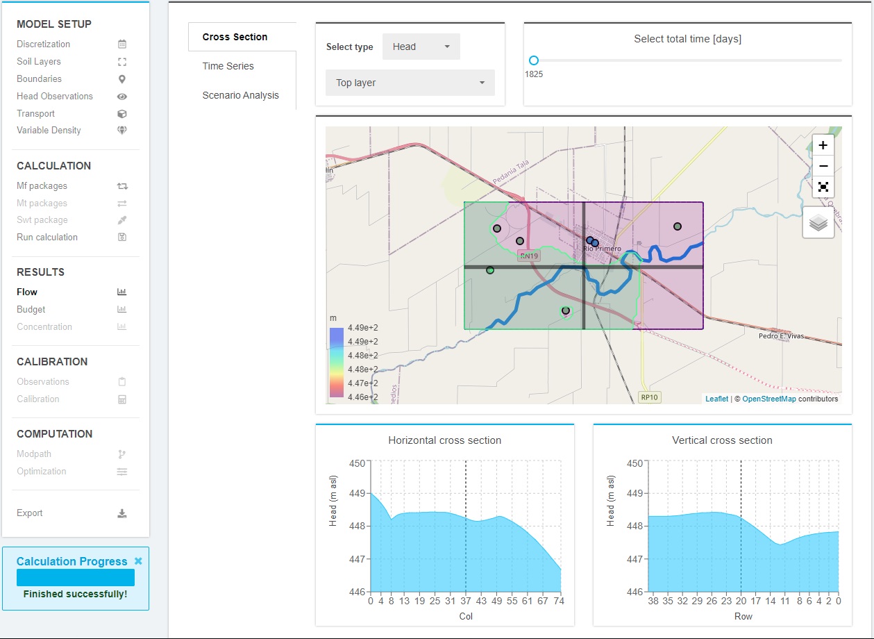
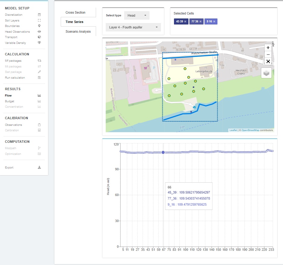
Time series
The time series of specific cells can be viwed by clicking on the desired cell.
Scenario Analysis
By clicking on the scenario analysis slider, a scenario analysis can be created and the INOWAS tool “T07 MODFLOW Model Scenario Manager” is opened.
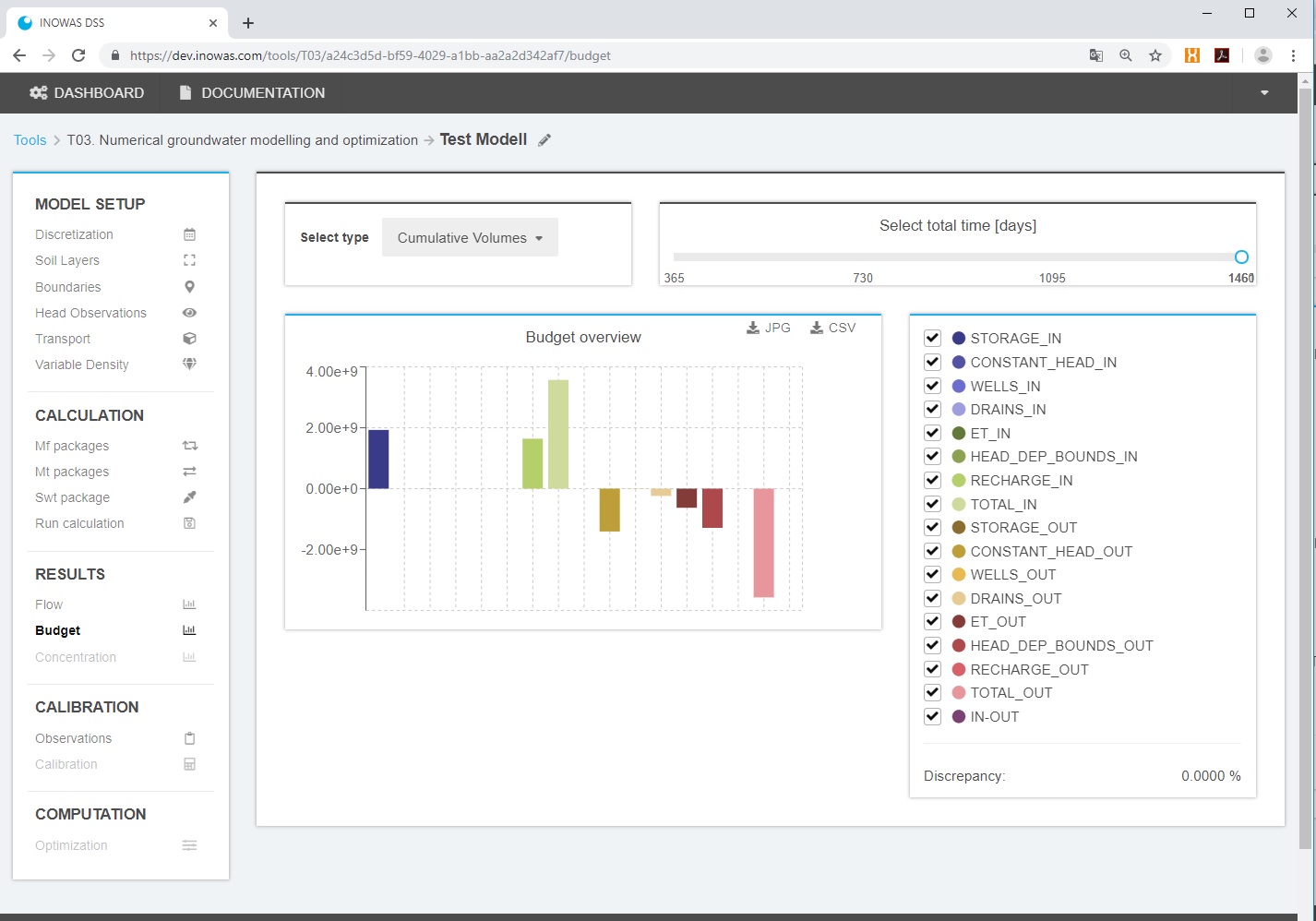
Budget
In the Budget results view, the cumulative volumes as well as the rates per time step can be displayed for the various stress periods. The boundary in and out fluxes and the total fluxes of the numerical groundwater flow model can be switched off and on to have a look at various components in detail. In addition, the percent discrepancy of the flow budget is given.
Calibration
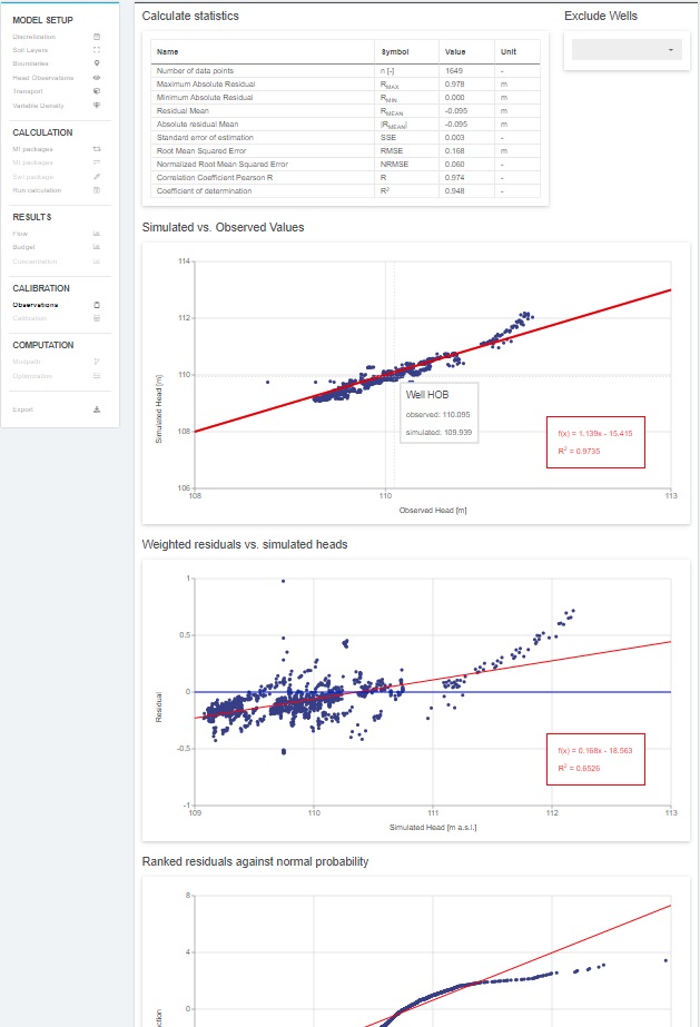
The calibration window currently includes the following functionalities to assess the quality of the model results:
- Visualize the calculated statistics
- Number of data points
- Maximum Absolute Residual
- Minimum Absolute Residual
- Residual Mean
- Absolute Residual Mean
- Standard error of estimation
- Root Mean Squared Error
- Normalized Root Mean Squared Error
- Correlation Coefficient Pearson R
- Coefficient of determination
- Graph visualising the simulated versus observed values
- Graph visualising the weighted residuals versus the simulated heads
- Graph visualising the ranked residuals against normal probability
SUPPORTED PACKAGES
The following MODFLOW-2005 packages are currently supported on the INOWAS platform:
| BAS6 | Basic Package |
| DIS | Discretization File |
| LPF | Layer-Property Flow Package |
| BCF6 | Block-Centered Flow package |
| CHD | Time-Variant Specified-Head Package |
| FHB | Flow and Head Boundary Package |
| RCH | Recharge Package |
| WEL | Well Package |
| GHB | General Head Boundary Package |
| OC | Output Control |
| RIV | River Package |
| DRN | Drain Package |
| EVT | Evapotranspiration Package |
| PCG | Preconditioned Conjugate-Gradient Package |
| DE4 | Direct Solver Package |
The implementation of further MODFLOW-related packages is planned. In addition, solute transport using MT3DMS (see T03b. Solute transport (MT3DMS)) can be added to the simulation. The implementation of density-driven flow (SEAWAT) with the relevant packages will be integrated soon.
TUTORIALS
Download our two tutorials and learn step-by-step how to use the INOWAS tool “T03.Numerical groundwater modelling and optimization” for your project.
- Tutorial 1. How to setup a steady state groundwater flow model. Read more.
- Tutorial 2. Transient groundwater flow model and scenario analysis. Read more.
External Links
For more information on the individual packages and program functionalities, see the USGS MODFLOW website, the Online Guide to MODFLOW-2005 or Harbaugh, 2005.
References
-
- Bakker, M., Post, V., Langevin, C.D., Hughes, J.D., White, J.T., Starn, J.J., Fienen, M.N., 2016. Scripting MODFLOW Model Development Using Python and FloPy. Groundwater 54, 733–739. doi:10.1111/gwat.12413
- Darcy, H., 1856. Les fontaines publiques de la ville de Dijon: exposition et application… Victor Dalmont.
- Harbaugh, A.W., 2005. MODFLOW-2005, the US Geological Survey modular ground-water model: the ground-water flow process (No. 6-A16), U.S. Geological Survey Techniques and Methods. US Department of the Interior, US Geological Survey Reston, VA, USA; online available: https://pubs.usgs.gov/tm/2005/tm6A16/.
- Hesch, W., Chmakov, S., 2011. A Unified Modeler’s Workbench: Workflow-Driven Conceptual and Numerical Modeling, in: Proceedings ModelCARE2011 Held at Leipzig, Germany, in September 2011.
- Ringleb, J., Sallwey, J., Stefan, C., 2016. Assessment of Managed Aquifer Recharge through Modeling—A Review. Water 8, 579. doi:10.3390/w8120579