Selection of suitable sites is an essential part of planning and conducting a sustainable and efficient MAR project. This tool combines GIS based geospatial analysis with multi-criteria decision analysis which is increasingly being used for MAR suitability analysis.
Multi-criteria decision analysis (MCDA) has been combined with geographical information systems (GIS) for solving geospatial problems to numerous scientific areas. The combination of both approaches is called geographical information systems multi-criteria decision analysis (GIS-MCDA). The tool includes a step-by-step approach to perform GIS-MCDA for MAR suitability analysis through a web-GIS and supporting tools. The process of MCDA for site selection follows the scheme developed in Rahman et al. (2012) and is divided into:
- problem definition,
- screening of feasible areas (constraint mapping),
- suitability mapping including the classification of thematic layers or criteria, standardization, weighting of the criteria and layers overlaying,
- sensitivity analysis.
Not all steps have to be included into the suitability analysis process, e.g. constraint mapping can be skipped depending on available data and problem definition.
A supplementary tool providing some historical background on the use of GIS-MCDA in the context of MAR suitability analysis is available. For this, a literature review was conducted compiling scientific studies on this topic. The results of the assessment of said studies are presented to aid the user in the decision on which criteria to use, how to standardize the selected criteria and which weights to assign during the combination. The resulting database along with a query tool can be found here: Go to database.
There are vast options of software and tools to perform the tasks included in GIS-based MCDA. The navigation on the left-hand side of the tool shows the single steps (Figure 1). Steps may be deactivated due to unmet conditions. In this case it shows a small yellow exclamation mark. When hovering over it, it shows the reason, why the step is still disabled.
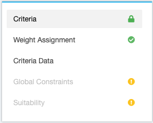
Figure 1 Tool navigation
0. Problem definition
Before commencing with GIS-MCDA the user needs to define and characterize the problem he wants to solve. Typical questions that need to be answered in this step are:
- What MAR method is proposed?
- What is the purpose of the MAR application?
- What is the source of the infiltration water?
- Which data is available to the user?
The problem definition outlines the whole MCDA process. Based on this information the criteria for the GIS analyses are chosen. The data available also defines whether a constraint map or a suitability map is applicable. In order to help the user with outlining the problem, a separate help page has been designed that concludes data from previous MCDA-GIS studies (Database)
1. Criteria
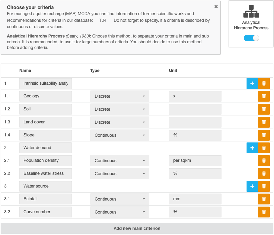
Figure 2 Criteria and Analytical Hierarchy Process
1.1 Hierarchy of criteria and sub-criteria
The process of grouping the used criteria into sub-criteria and main criteria is only relevant if the user chooses to use Analytical Hierarchy Process (AHP) for the assignment and combination of weights. It was proposed by Saaty (1980) and should be used for MCDA analysis with a large number of criteria. The chosen criteria set (see section 1.2) is taken with each criterion initially set as a sub-criterion. Sub-criteria are then grouped under main criteria and the combined main criteria ultimately form the suitability map. In this way a three-level hierarchy system is being built (Figure 3). The criteria tree is used to aid the user in assigning weights in a more structured and robust way.
In the first step of the tool, AHP can be activated or deactivated by clicking on the small slider on the top-right of the page (Figure 1).
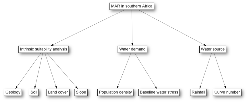
Figure 3 Example for criteria hierarchy in Analytical Hierarchy Process
1.2. Choice of criteria and sub-criteria
From the data that is available a criteria set needs to be chosen to generate the GIS maps. Again, it might be helpful for the user to compare his situation to previous GIS studies which may aid in finding the criteria that are most suitable for his problem (Database). The criteria set should be complete, operational, decomposable, non-redundant and minimal. Each criterion has to be compressive and measurable (Malczewski, 1999). The criterion can be used in constraint mapping, suitability mapping or both. The value of the criterion can vary between the constraint and suitability mapping. The spatial distribution of each criterion has to be coincident with the study area (complete criteria set). The criterion with the minimum resolution or scale will define the scale of the final result. A criterion could be either a discrete (divided into classes) or continuous variable.
Criteria that are typically used for GIS-MCDA in the context of MAR are: geology, lithology, land use, slope, and soil texture. For constraint mapping also distances to sources or water users, protected areas or potential hazards are considered. An overview about all previously used criteria can be found here (Database).
If AHP is not active, criteria can be added by clicking on “Add new criterion”. With AHP, main criteria can be added in the same way. Sub-criteria are added then by clicking the “Add sub-criterion” button of the appropriate main criterion. For each criterion or sub-criterion (if AHP is active), it must be selected, if the criterion’s data is continuous or discrete. Furthermore, a unit can be entered for each criterion. The units will appear in map legends and have only a visualization purpose.
2. Weight Assignment
The assignment of different weights to the criteria is necessary as not all of them have the same degree of influence on the MAR applicability and thus should be weighted accordingly during the integration of suitability maps. There are several methods to assign weights to the criteria. The following methods are described further in this introduction: Rating method, Ranking method, Multi-influence factor method and Pairwise comparison. Weighting methods vary in terms of easiness to use and theoretical foundation.
Within the tool, the user can perform any number of weigh assignments for each set of criteria by selecting the desired method on the left side (figure 4). This can be useful, for analysing different scenarios. Before starting the calculation in step 5, the user must select, which weight assignments out of the performed ones, are going to be used.
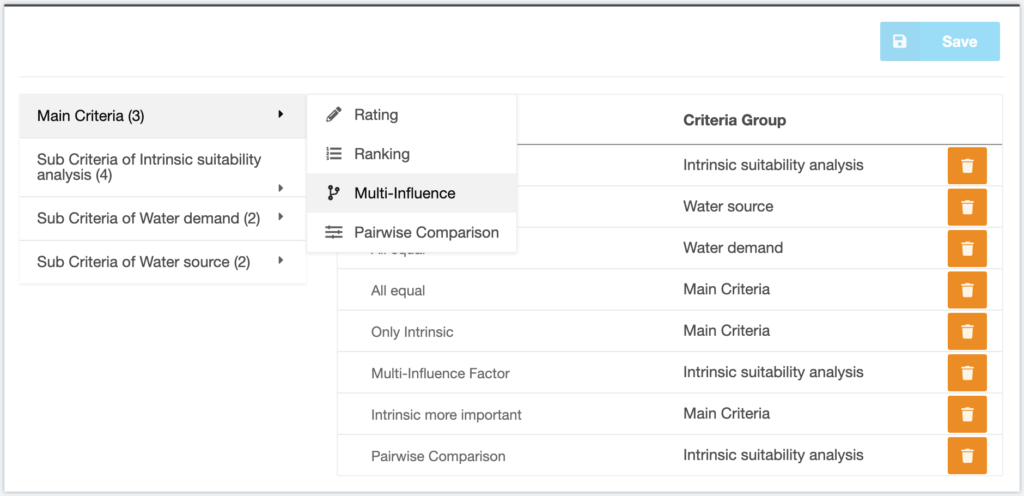
Figure 4 Weight assignment main menu with different weighting scenarios
2.1 Rating method
The weights are assigned based on the user knowledge. This option is called expert criteria and can be based on the knowledge of the user or comparison to previous studies (Database). The highest score is assigned to the most important criterion. This is then done proportionally for all criteria. The user can choose the range of scores freely. The weights are calculated out of the entered scores in relation to the sum of all scores.
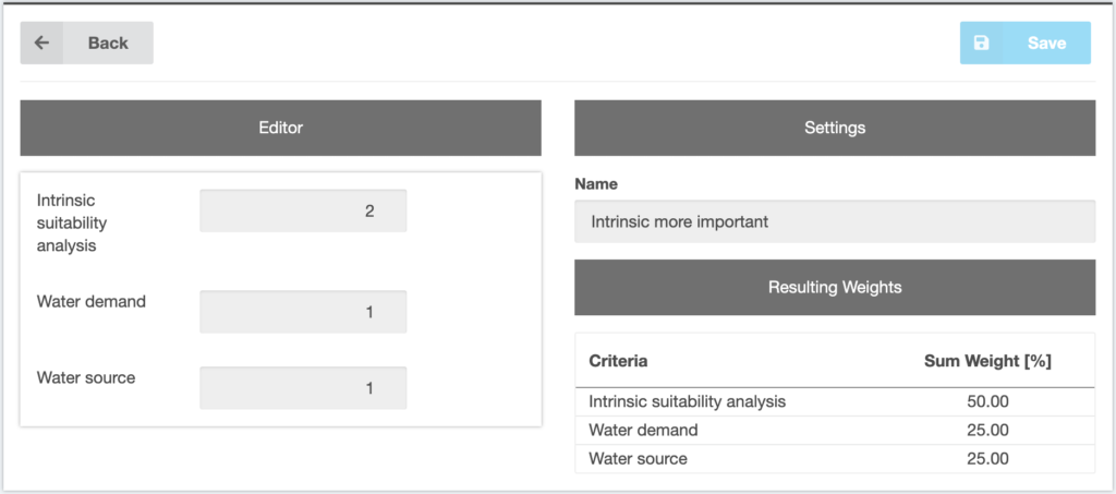
Figure 5 Rating method menu
This method lacks theoretical foundation. It is, however, very easy to apply and widely used.
2.2 Ranking method
The criteria are assigned a rank. The most important criterion is ranked the first and the least important ranked last. The rank sum weights can be calculated according to equation 1:
| w_{k}= \frac{n-p_{k}+1}{ \sum_{k=1}^{n}(n-p_{k}+1)} | (eq. 1) |
where wk is the k-th criterion weight, n is the number of criteria under consideration (k=1,2,…,n) and pk is the rank position of the criterion.
Other ways to calculate the weights is by using the rank reciprocal (eq.2) which puts more emphasis on the most important criterion, or rank exponent methods (eq.3).
| w_{k}= \frac{1/p_{k}}{ \sum_{k=1}^{n}1/p_{k}} | (eq. 2) |
| w_{k}= \frac{(n-p_{k}+1)^{z}}{\sum_{k=1}^{n}(n-p_{k}+1)^{z}} | (eq. 3) |
where z is the exponent.
Within the tool, the criteria can be ordered via drag and drop or by clicking on the arrow buttons next to them (Figure 6). On the right-hand side of the screen, the user may select the desired mathematical function: rank sum weights, rank reciprocal or rank exponent, where the exponent has to be entered as well.
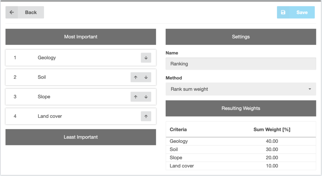
Figure 6 Ranking method menu
The method is simple and has been widely used (Malczewski and Rinner, 2015). It does, however, lack theoretical foundation. Furthermore, the larger the criteria set, the less useful is the ranking method.
2.3 Multi-influence factor method (MIF)
This method has been described by (Magesh et al., 2012; Shaban et al., 2005). The weights are assigned by plotting the criteria and their relationships or rather the effect between each of them (Figure 7). The estimation of the weights of each criterion is based on the effect that they have among each other with the differentiation of major effects (score of 1) and minor effects (score of 0.5). The final criterion weight is the cumulative score of both major and minor effects.
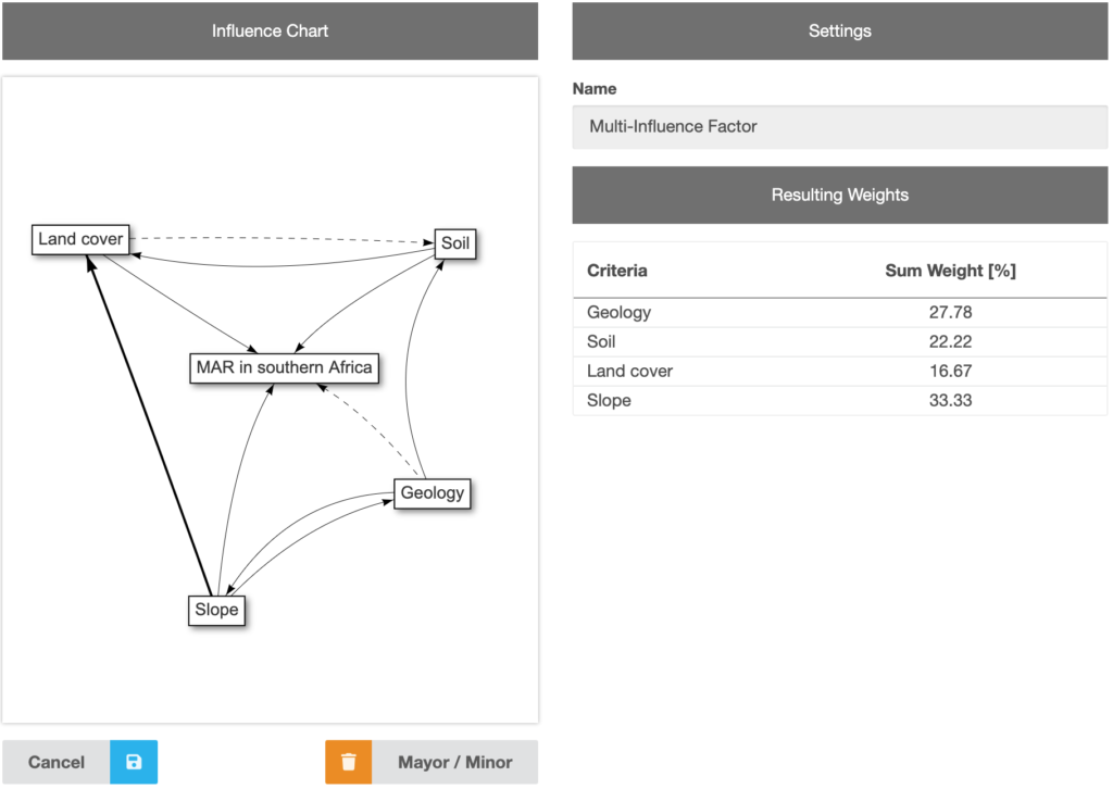
Figure 7 Multi-influence factor menu showing an example with interrelationships between the different criteria affecting the MAR suitability in southern Africa.
The interrelations need to be drawn and defined by the user and separated by the importance of the effect. The scores are then added and the weight is calculated according to table 1.
Table 1 Effect of influencing factor, relative rates and score for each potential factor
| Factor | Major effect (A) | Minor effect (B) | Proposed relative rates (A+B) | Proposed score of each influencing factor |
| Land cover | 1 | 0.5 | 1.5 | 16.67 |
| Soil | 1+1 | 0 | 2.0 | 22.22 |
| Geology | 1+1 | 0.5 | 2.5 | 27.78 |
| Slope | 1+1+1 | 0 | 3.0 | 33.33 |
The proposed final score is calculated using equation 4.
| \left [\frac{(A+B)}{\sum (A+B)} \right ]*100 | (eq. 4) |
This method is easy to understand and very visual. It has a stronger theoretical foundation than the rating and ranking method.
A tool for the MIF method is provided (Figure 7). Clicking on the “Start Editing” button on the bottom left, the editing mode is being activated. By clicking on a node and holding the mouse key, moving the cursor to another node and releasing the mouse key there, an influence arrow can be drawn between two nodes. An arrow can be deleted or changed to a minor influence, by clicking on it and using the buttons on the bottom right of the editor. After all influences are drawn and minor/major effects are specified, the small blue save button (floppy icon) has to be clicked in order to calculate the cumulative score as well as relative weight of each factor.
Criteria can be connected to the project node, to show their influence on the problem itself. This is useful for instance, if one criterion is not regarded by the MIF method because it is only influenced by other criteria but it doesn’t influence criteria itself but the user still wants to consider that criterion in the rating.
If the editing mode is not active, the nodes can be dragged around in order to provide better visibility. By right clicking on the editor area, the network can be saved as an image.
2.4 Pairwise comparison
The assignment of weights is based on the pairwise matrix by Saaty (1980) and is based on rating the preference of a pair of criteria and creating a ratio matrix. It aids in calculating the weights as well as the consistency ratio which indicates the consistency of the pairwise judgement.
At first the pairwise comparison matrix has to be defined. Based on the scale presented in table 2 the preference for each criterion has to be defined in pairwise comparison. As an example we will conduct pairwise comparison for the three criteria slope, land use and drainage intensity.
Table 2 Pairwise comparison scale (Saaty, 1980)
| Defintion (importance) | Intensity of importance |
| Equal | 1 |
| Equat to moderate | 2 |
| Moderate | 3 |
| Moderate to strong | 4 |
| Strong | 5 |
| Strong to very strong | 6 |
| Very strong | 7 |
| Very to extremely strong | 8 |
| Extreme | 9 |
To compare all criteria n*(n-1)/2 comparisons need to be made. In this example three comparisons are sufficient. Out of these comparison values a matrix is created that shows the comparison values of all the criteria towards each other (Table 3). The comparison matrix is reciprocal which means that if land use receives a score of 3 compared to drainage intensity, drainage intensity in return receives the reciprocal value 1/3 compared to land use.
Table 3 Comparison matrix for pairwise comparison of the criteria set
| Criterion | Drainage intensity | Land use | Slope |
| Drainage intensity | 1 | 3 | 6 |
| Land use | 1/3 | 1 | 3 |
| Slope | 1/6 | 1/2 | 1 |
From the comparison matrix the criterion weights are computed. This computation involves three steps: (1) sum the values of each column of table 3; (2) divide each element of the matrix by its column total (the result is called normalized pairwise comparison matrix) and (3) compute the average of the elements of each row of the normalized matrix. These averages are an estimate of the relative weights of each criterion (Table 4).
Table 4 Normalized comparison matrix and calculated weight for each criterion
| Criterion | Drainage intensity | Land use | Slope | Weight |
| Drainage intensity | 0.66 | 0.66 | 0.6 | 0.64 |
| Land use | 0.22 | 0.22 | 0.3 | 0.25 |
| Slope | 0.11 | 0.11 | 0.1 | 0.11 |
After computing the weights, the consistency of the comparisons is assessed. To do so, the weighted sum vector needs to be determined by multiplying the weight of the first criterion times the first column of the original comparison matrix (Table 3). The other columns are handled accordingly and the sums of the rows are calculated. This weighted sum vector is then divided by the criterion weights; the result being the consistency vector (Table 5).
Table 5 Steps for determining the consistency ratio
| Criterion | Weighted sum vector | Consistency vector |
| Drainage intensity | 0.64*1+0.25*3+0.11*6=2.05 | 2.05/0.64=3.2 |
| Land use | 0.64*1/3+0.25*1+0.11*3=0.79 | 0.79/0.25=3.16 |
| Slope | 0.64*1/6+0.25*1/2+0.11*1=0.45 | 0.45/0.11=4.09 |
With the consistency vector the consistency ratio can now be calculated (eq. 5):
| CR=\frac{\lambda -n}{RI(n-1)} | (eq. 5) |
with n is the number of criteria, lambda is the average of the consistency vector and RI is a random index whcih depends on the number of criteria used (Table 6).
Table 6 Random consistency index (Saaty, 1980)
| n | RI |
| 1 | 0 |
| 2 | 0 |
| 3 | 0.56 |
| 4 | 0.90 |
| 5 | 1.12 |
| 6 | 1.24 |
| 7 | 1.32 |
| 8 | 1.41 |
| 9 | 1.45 |
| 10 | 1.49 |
| 11 | 1.51 |
| 12 | 1.48 |
| 13 | 1.56 |
| 14 | 1.57 |
| 15 | 1.59 |
If the consistency ratio (CR) is less than 0.1 a reasonable level of consistency in the pairwise comparison matrix is indicated. Thus, if CR is >= 0.1 the pairwise comparison should be reconsidered as the comparisons are inconsistent. For this example the CR is 0.42, thus, the pairwise comparisons should be reconsidered. By changing the score of slope compared to land use only slightly from 3 to 2, the consistency ratio generates a satisfying value.
A detailed description of pairwise comparison can be found in Malczewski (1999, p.182). This method is more complex and is based on a theoretical foundation (statistical/heuristic). It is still relatively easy to use and understand. The nature of the pairwise comparison is easy to comprehend as only two criteria are considered at a time. However, if many criteria are compared (n=10) then the number of pairwise comparisons (45 in that case) can be time-consuming. This method has been tested to be one of the most effective techniques for MCDA (Malczewski, 1997).
A tool is available to compute the weights as well as the consistency ratio (Figure 8). All criteria are compared with each other, by moving a slider between them. If the slider is in the middle, both criteria are considered to be equally important (value 1). If the slider is on the left side, the left criterion is more important than the right one and if the slider is on the right side, the right criterion is more important than the left one.
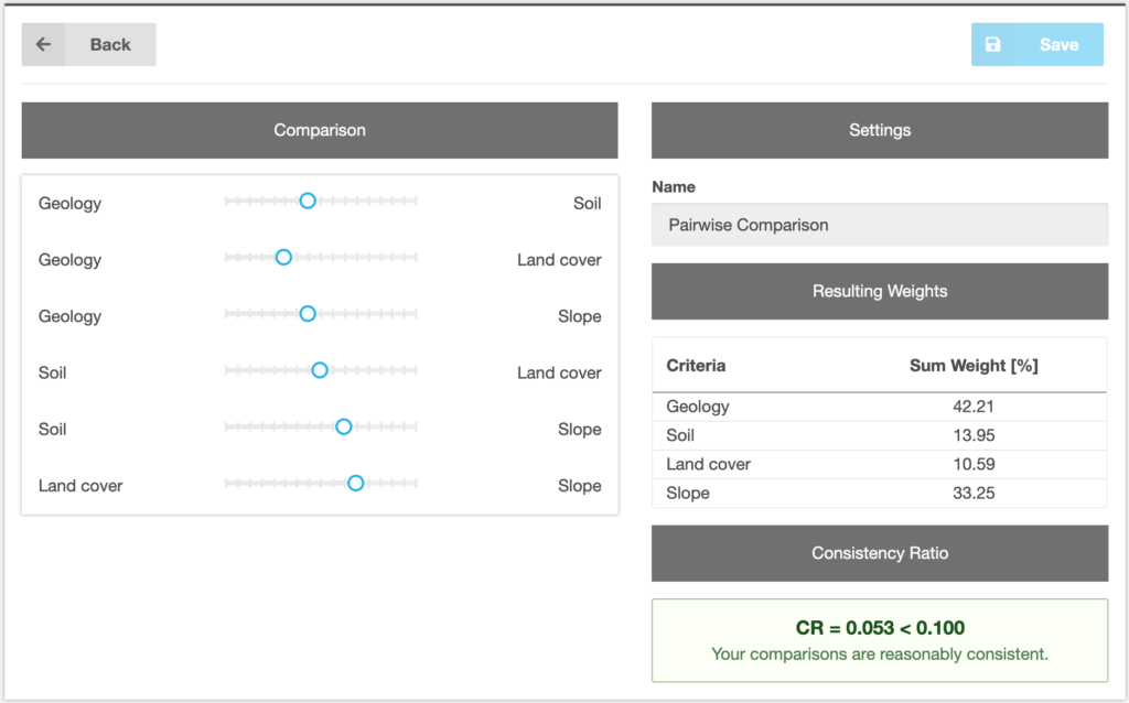
Figure 8 Pairwise comparison menu
3. Data upload and GIS
When entering the third step inside the tool, a second navigation appears on the left-hand side (Figure 9). The first step must be the selection of the desired grid size. It not only defines the output grid size of the suitability map, but also the size to which all uploaded raster files are going to be interpolated. Higher grid sizes may result in higher loading times, depending on the users’ hardware. The second part of the navigation is a list of the previously added criteria. The steps explained below have to be done for each criterion by selecting them from the list. When they are fulfilled, a green exclamation mark is displayed next to the criteria.
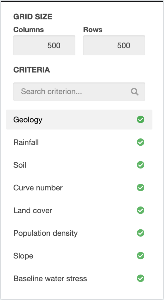
Figure 9 Criteria navigation
On the top of the right side of the tool, another horizontal navigation guides the user through the single steps necessary for the data handling (Figure 10). Some steps are not accessible before a certain condition has been met.

Figure 10 Criteria data and GIS navigation
3.1 Criteria upload
By clicking the “Upload Raster File” button, a modal opens, where users can select an interpolation order and a file to be uploaded from their hard drive (Figure 11). It is recommended to select the “Nearest-neighbor” interpolation or “No interpolation”, if the file already has the correct grid size. If the file is valid, it shows some metadata on the top-right, the different color bands on the bottom-left and a preview on the bottom-right. By clicking on the blue apply button, the data is going to be stored and the constraints and reclassification step become available.
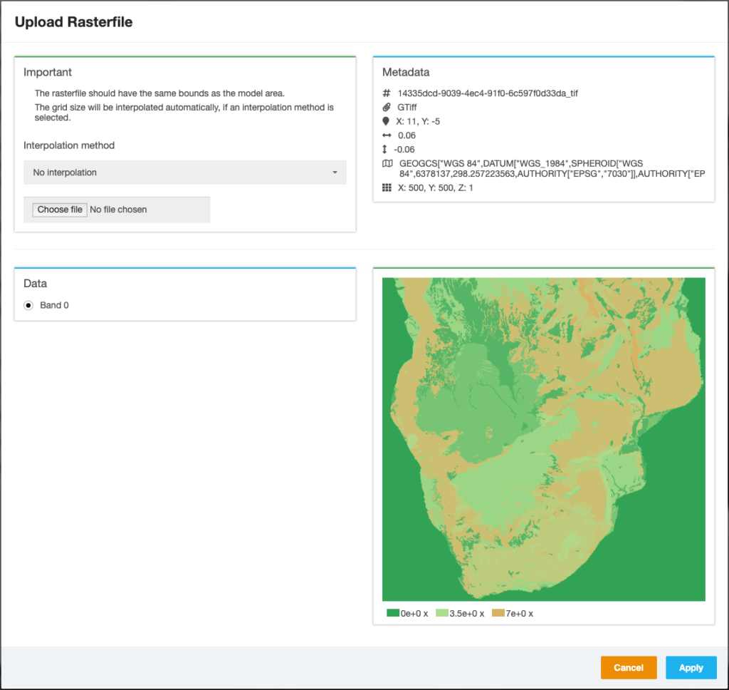
Figure 11 Criteria data upload modal
3.2 Constraint mapping
The main idea of constraint mapping is the elimination of parts of the study area that are not feasible for application of MAR. The reasons for non-feasibility can be manifold: proximity to water source, protected areas, land that is not available (private owners), etc. Thus, the user needs to define the constraint criteria and the threshold value of each criterion. It is recommended that the areas where the criterion is suitable are assigned with a value of 1 and the areas that are not suitable a value of zero. After doing this for all criteria, the layers are merged with Boolean logic meaning that all areas with a value of 0 after the integration of the constraint criteria are unsuitable, and all the areas with a value of 1 are suitable. The suitable areas should be further analysed through suitability mapping.
In the tool, there are two possibilities of defining constraints. They can be set either depending on the criteria data or globally for the whole project (see step 4). Defining constraints for criteria is different for discrete and continuous data. In the constraint mapping menu (Figure 12), on the right side, it shows the resulting constraints map. Red color stands for unsuitable cells (value 0) and green color for suitable cells (value 1). For discrete data, all existing classes are listed on the left side and can be defined as constraint by deactivating the small sliders (figure 12).
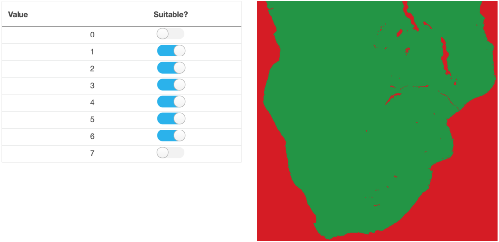
Figure 12 Constraint mapping for discrete criteria data
For continuous data, constraint rules can be added by clicking on the blue “Add Rule” button (Figure 13). Each rule is characterized by an interval, which can be entered by selecting a minimum and a maximum value and comparative operators. All raster cells with values inside of those intervals are defined as constraints. It is necessary to click on the “Recalculate Raster” button on the right side, to apply the constraints rules. The step of constraint mapping is optional and can be skipped.

Figure 13 Constraint mapping for continuous criteria data
3.3 Reclassification and Standardization
In order to reduce the dimensionality of the different criteria and combine them, they have to be converted into a common scale. The standardization is based on the fuzzy method, meaning that for each layer all geodata is reclassified and is assigned a value between 0 and 1 (the higher the value, the more suitable). Classification has to be done for each layer individually and is based on the content of the layer. Classification can be based on numerical values or linguistics- such as good, moderate, bad. Step-wise and linear functions are the most common standardization methods. Different methods may be applied to different criteria maps. Within the literature review a section covers commonly used standardization methods for the criteria that are used most for MAR suitability mapping (Database).
Step-wise functions (Figure 14) can be applied analogously to constraint mapping. The only difference is that more than two classes can be defined and applied.

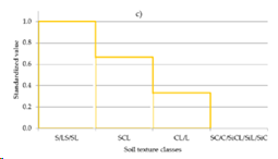
Figure 14 Example of step-wise standardization (Bonilla et al., 2016)
Standardization functions can have different shapes and need to be applied by defining ranges and their respective function. Usually these functions have to be defined by the user with the help of literature references or experience. An example for the conversion of a more complex standardization function is given below for the case of terrain slope (taken from Bonilla et al., 2016).
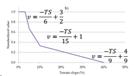
Figure 15 Example of linear standardization (Bonilla et al., 2016)
In the tool, the reclassification process is different for discrete and continuous data, similar to the constraints step. For discrete criteria, all existing classes are listed on the right side. Each class can be customized by a colour, a name and the standardized value (Figure 16).
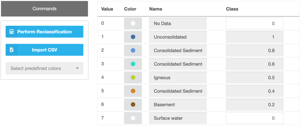
Figure 16 Standardization of discrete criteria data
For continuous data, classes can be added by clicking on the “Add Class” button on the left side (Figure 17). It opens a modal, where users can edit the color and name of the class as well as the interval, which defines the class range and the standardized value or applied function (Figure 18). Functions can be used to calculate a linear relationship between original and standardized values. Classes can be edited or deleted by clicking on the grey buttons on the right side. The chart on the bottom visualizes the standardized values.
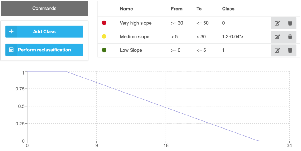
Figure 17 Standardization of continuous criteria data
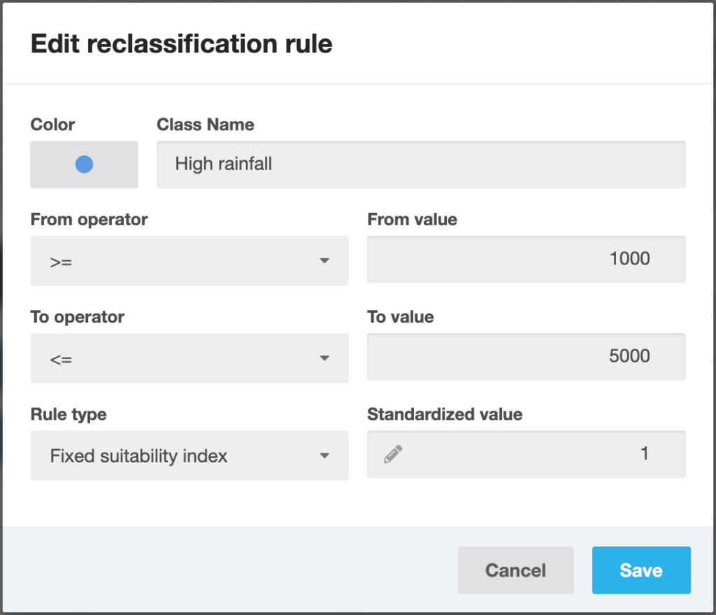
Figure 18 Modal for creating and editing classes for continuous criteria data
It is necessary to click on the blue “Perform reclassification” button on the left side, to proceed.
3.4 Results
After the reclassification has been done, the last step becomes available. This one is just for visualization of the results. The layers can be shown in the map: the reclassified and standardized data (Suitability), the original raster (Criteria Data) and the constraints. The classes created in the previous step can be shown by selecting “Criteria Data” and the “Reclassified” colour scheme (figure 19). If the grid size of the project exceeds a certain size, the rasters are shown as images and not on top of the Leaflet map. To switch to the map, the “Show on map” button above the image can be clicked. It may take some time to render the map depending on the users’ hardware.
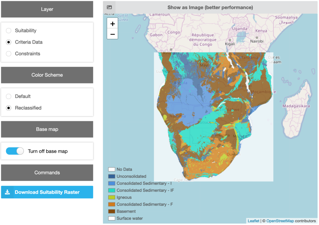
Figure 19 Results view showing the reclassified data
4. Global constraints
The global constraints step is optional and can be skipped, if no global constraints have to be set. Users can draw polygons in the map, which are going to be excluded from the final suitability calculation (Figure 20). By clicking on the big grey button above the map, the editing mode starts. Constraint polygons are defined by clicking on the map and adding edge points. The constraint raster will be created by clicking on the blue “Cut and Process” button on the left side.
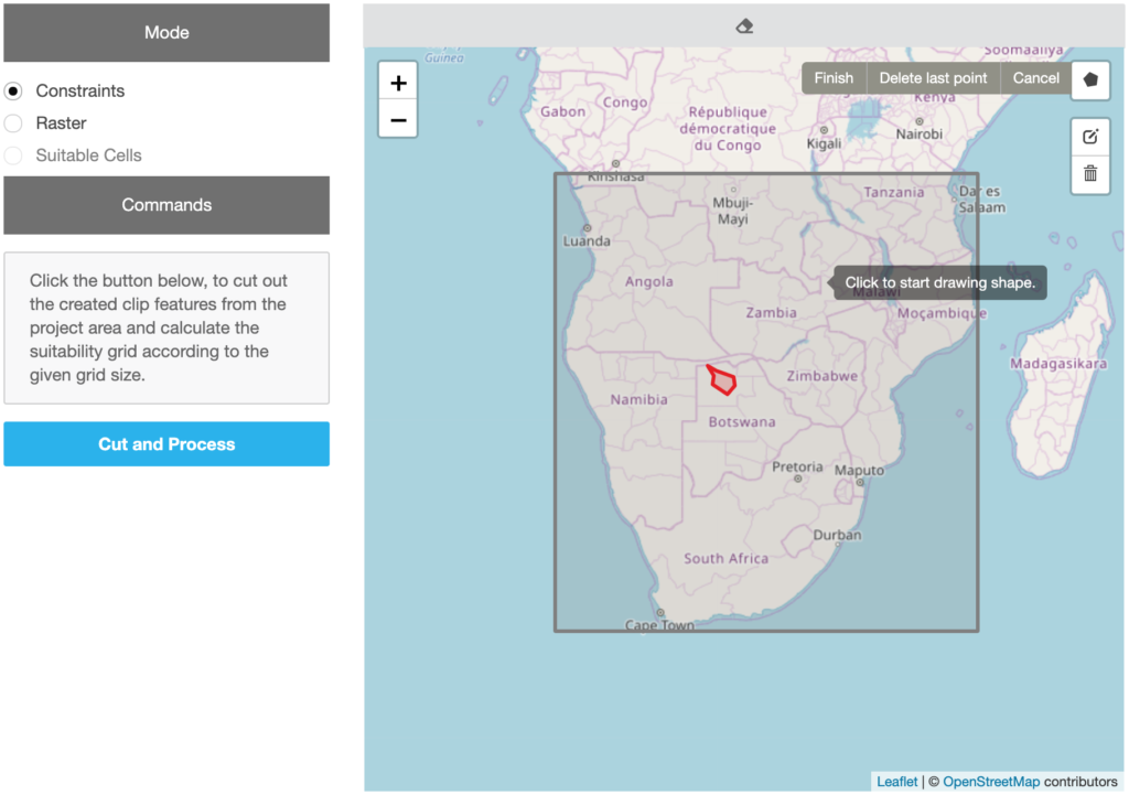
Figure 20 Adding constraint polygons
5. Suitability
After the weights for the criteria have been set, these elements have to be combined by applying decision rules. Decision rules dictate how to best order alternatives or to decide which alternative is preferred to another. It is the integration of datasets and weighting preferences.
Weighted linear combination (WLC) is one of the most popular decision rules. WLC is based on the weighted average concept in which the weight of “relative importance” of each criterion is assigned by the decision maker. The suitability of a site is obtained by summing up all the products of the standardized criteria maps multiplied by their respective weights (eq. 6).
| A_{i}=\sum_{j}w_{j}x_{ij} | (eq. 6) |
with xij=score of the i-th alternative with respect to the j-th criterion
wj= normalized weight of criterion
Like in step 3, a horizontal navigation guides users through the process (Figure 21).

Figure 21 Navigation of the suitability calculation step
5.1. Select weight assignment methods
Before users can start the final suitability calculation by clicking on the blue “Start Calculation” button, they have to select the weight assignment methods to be used. If the AHP process had been activated in step 1, a method has to be selected for each set of sub criteria and the main criteria (Figure 22). If AHP is not active, just one weight assignment is necessary.
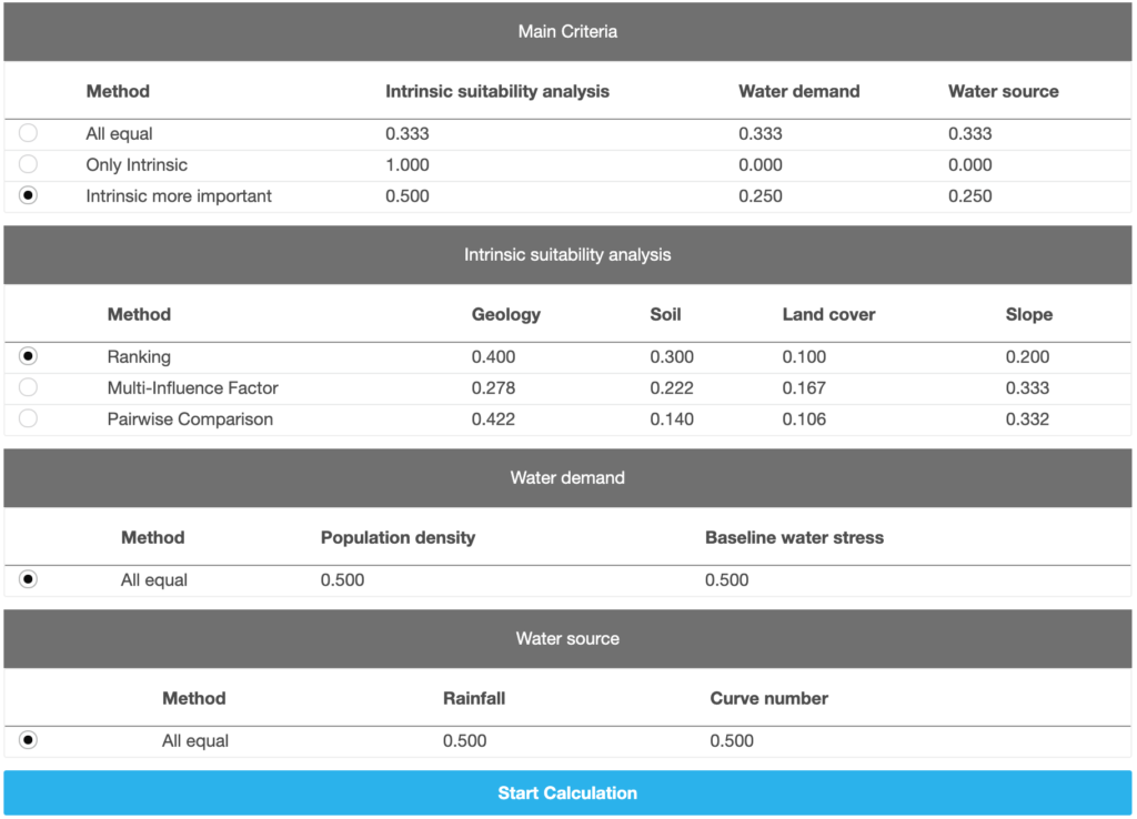
Figure 22 Selecting weight assignment methods
5.2 Suitability classes
The suitability classes are predefined but can be changed in the “Classes” step (Figure 23). This is done in the same way, like the classes being created for continuous data in step 3 (see 3.3).
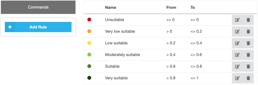
Figure 23 Defining suitability classes
5.3 Final result
The final result can be seen by clicking on the “Results” step in the top navigation after the calculation has been finished (Figure 24) . The view is similar like the one for the criteria data explained in 3.4 . The final raster can be downloaded as an ASCII-file by clicking on the “Download Raster” link on the bottom left.
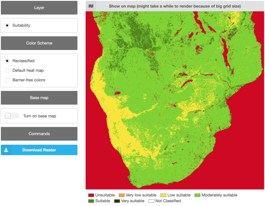
Figure 24 Final results view
6. Perform a sensitivity analysis
Because the criterion values and weights are the main sources of uncertainty in the GIS-MCDA, conducting a sensitivity analysis allows for more robust decision making. Sensitivity analysis is used to showcase the effect of different criterion weights on the spatial pattern of the suitability map. Methods and instructions for the sensitivity analysis are available in Malczewski (1999, p.261). The effect of criterion weights can be analyzed by changing the weights one at a time and evaluating its influence on the resulting map. This can be done by changing the weights manually or adjusting the weighting method used, e.g., in case of using the MIF methods by adding or deleting interrelations between the criteria. With the changed weights a new suitability map is generated. Suitability maps for each new scenario (=changed weight) need to be compared to the original suitability map. Using the same suitability classes for each map, the newly generated maps for each scenario should be subtracted from the original map. Thus, for each scenario a raster with positive and negative values is created. A positive value stands for the change of a higher to a lower class and a negative value stands for the change of a lower to a higher class. Positive and negative changes have no relation to the effect but they showcase the robustness of the chosen weights. The smaller the differences, the more robust are the chosen weights.
This step is not yet included into the web-tool but a online implementation is envisioned.
REFERENCES
- Bonilla, J., Blank, C., Roidt, M., Schneider, L., Stefan, C., 2016. Application of a GIS Multi-Criteria Decision Analysis for the Identification of Intrinsic Suitable Sites in Costa Rica for the Application of Managed Aquifer Recharge (MAR) through Spreading Methods. Water 8, 391.
- Magesh, N.S., Chandrasekar, N., Soundranayagam, J.P., 2012. Delineation of groundwater potential zones in Theni district, Tamil Nadu, using remote sensing, GIS and MIF techniques. Geosci. Front. 3, 189–196. https://doi.org/10.1016/j.gsf.2011.10.007
- Malczewski, J., 1999. GIS and multicriteria decision analysis. John Wiley & Sons.
- Malczewski, J. (1997). Propagation of Errors in Multicriteria Location Analysis: A Case Study. In: Fandel, G., Gal, T. (eds) Multiple Criteria Decision Making. Lecture Notes in Economics and Mathematical Systems, vol 448. Springer, Berlin, Heidelberg. https://doi.org/10.1007/978-3-642-59132-7_17
- Malczewski, J., Rinner, C., 2015. Multicriteria decision analysis in geographic information science. Springer. https://doi.org/10.1007/978-3-540-74757-4
- QGIS Development Team, 2016. QGIS User Guide. Release 2.14., Open Source Geospatial Foundation Project.
- Rahman, M.A., Rusteberg, B., Gogu, R.C., Lobo Ferreira, J.P., Sauter, M., 2012. A new spatial multi-criteria decision support tool for site selection for implementation of managed aquifer recharge. J. Environ. Manage. 99, 61–75. https://doi.org/10.1016/j.jenvman.2012.01.003
- Saaty, T.L., 1980. The analytical hierarchial process. McGraw-Hill, New York.
- Shaban, A., Khawlie, M., Abdallah, C., 2005. Use of remote sensing and GIS to determine recharge potential zones: the case of Occidental Lebanon. Hydrogeol. J. 14, 433–443. https://doi.org/10.1007/s10040-005-0437-6