The tool uses the analytical solution of the advection-dispersion equation according to Ogata and Banks to determine the concentration of a contaminant down-gradient from a constant source, at a given distance x and time t under consideration of one-dimensional transport in a homogeneous and isotropic porous aquifer with a constant velocity along the flow direction. The transport of the contaminant under consideration of retardation can be calculated optionally.
The knowledge about contaminant concentration distribution behavior along groundwater flow is of importance for management of water infiltrated by MAR applications. Besides a lot of numerical models, analytical models exist to describe the solute transport in groundwater. Assuming primarily one dimensional transport where solute concentration is horizontally and vertically well mixed so that concentrations vary only in the longitudinal or downstream direction, the advection-dispersion equation (equation 1) is a suitable model to describe the transport of solutes in groundwater.
| (eq. 1) |
where
| C | = Concentration of the solute in the fluid [ML-3] |
| t | = Time since introduction of constant point concentration [T] |
| DL | = Longitudinal dispersion coefficient [L2T– 1] |
| x | = Down gradient distance from constant point concentration [L] |
| vx | = Down gradient average fluid velocity [LT– 1] |
Initial and boundary conditions are:
Ogata and Banks (1961) developed an analytical solution of the advection-dispersion equation under assumption of the initial and boundary conditions for a conservative substance (no sorption, no degradation) in a homogeneous, porous medium.
| (eq. 2) |
where
| C | = Concentration of the solute in the fluid [ML-3] |
| C0 | = Initial (t=0) concentration of the solute in the fluid [ML-3] |
| DL | = Longitudinal dispersion coefficient [L2T– 1] |
| vx | = Down gradient average fluid velocity [LT– 1] |
| x | = Down gradient distance from constant point concentration [L] |
| t | = Time since introduction of constant point concentration [T] |
| erfc | = error function |
The 1D advection-dispersion equation, including the extension by retardation is given by equation 3:
| (eq. 3) |
where
| C | = Concentration of the solute in the fluid [ML-3] |
| t | = Time since introduction of constant point concentration [T] |
| DL | = Longitudinal dispersion coefficient [L2T– 1] |
| R | = Retardation factor [-] |
| x | = Down gradient distance from constant point concentration [L] |
| vx | = Down gradient average fluid velocity [LT– 1] |
The analytical solution of equation 3, developed by Bear (1972), is:
| (eq. 4) |
where
| C | = Concentration of the solute in the fluid [ML-3] |
| C0 | = Initial (t=0) concentration of the solute in the fluid [ML-3] |
| DL | = Longitudinal dispersion coefficient [L2T– 1] |
| vx | = Down gradient average fluid velocity [LT– 1] |
| x | = Down gradient distance from constant point concentration [L] |
| t | = Time since introduction of constant point concentration [T] |
| R | = Retardation factor [-] |
| erfc | = error function |
The online calculator needs user-supplied values for time of interest (t), location of interest (x) and a source concentration (C0) as well as transport properties velocity (vx), dispersion coefficient (DL) and retardation factor (R).
Down gradient average fluid velocity, vx
The average velocity by which groundwater is transported through the aquifer is caused by the hydraulic gradient and can be calculated according to equation 5 (Hölting and Coldewey, 2013).
| (eq. 5) |
where
| vx | = Down gradient average fluid velocity [LT– 1] |
| K | = Hydraulic conductivity [LT– 1] |
| ne | = Effective porosity [-] |
| I | = Hydraulic gradient [-] = |
Common ranges for effective porosity can be found in table 1 (Olshausen, 2013):
Table 1: Representative ranges for effective porosity
| Effective porosity [%] | |
| Clay | < 5 |
| Sand fine | 10 – 20 |
| Sand medium | 12 – 25 |
| Sand coarse | 15 – 30 |
| Sand gravelly | 16 – 28 |
Longitudinal dispersion coefficient, DL
Dispersion is describing the process of mechanical mixing that takes place in porous media as a result of movement of water through the pore space of soil. Under consideration of one dimensional transport the longitudinal dispersion is dominating. The longitudinal dispersion coefficient DLis a measure for this process and can be calculated according to equation 6 (Alvarez and Illman, 2005).
| (eq. 6) |
where
| DL | = Longitudinal dispersion coefficient [L2T– 1] |
| = Longitudinal dispersivity [L] | |
| vx | = Down gradient average fluid velocity [LT– 1] |
Longitudinal dispersivity αLdepends on the length of transport – the longer, the higher. Common values are in the range of 0.1 to 10 m.
Retardation factor, R
The movement of substances dissolved in groundwater is due to sorption processes different from the movement of groundwater. The retardation factor is describing the ratio of the groundwater velocity to the velocity of substances dissolved in groundwater and can be calculated according to equation 7 (Gillham et. al, 1982).
| (eq. 7) |
where
| R | = Retardation factor [-] |
| Kd | = Sorption partition coefficient [L3M-1] |
| |
= Bulk density [ML-3] |
| ne | = Effective porosity [-] |
The sorption partition coefficient describes the distribution of the substance between soil and water and can be determined in experiments depending on the organic carbon content of the soil. If no data is available, Kdcan be calculated according to empirical equation 9.
Bulk density, 
Bulk density of soils can be calculated according to equation 8 (Gillham et. al, 1982):
| (eq. 8) |
where
| |
= Bulk density [ML-3] |
| ne | = Effective porosity [-] |
| |
= Particle density [ML-3] |
A commonly used value for particle density for sandy material is 2.65 g/cm3 because of the density of the dominant mineral quartz. This means that a soil particle that is 1 cm3in volume weighs 2.65 g.
Sorption partition coefficient, Kd
If no data for Kdis available, the Sorption partition coefficient can be calculated according to equation 9 (Gillham et. al, 1982):
| (eq. 9) |
where
| Kd | = Sorption partition coefficient [L3M-1] |
| KOC | = Partition coefficient between organic carbon in the soil and water [L3M-1] |
| Corg | = Organic carbon content in the soil [MM] |
Partition coefficient organic carbon between soil and water, logKoc
Partition coefficient between organic carbon in the soil and water is calculated according to equation 9 (Karickhoff et. al, 1980).
| (eq. 10) |
where
| KOC | = Partition coefficient between organic carbon in the soil and water [LM-1] |
| KOW | = Octanol/water partition coefficient [LM-1] |
| a | = 1 (Constant according to Karickhoff et. al, 1979) |
| b | = 0.21 (Constant according to Karickhoff et. al, 1979) |
Octanol/water partition coefficient for a lot of organic substances can be found in Sangster, 1989.
Example
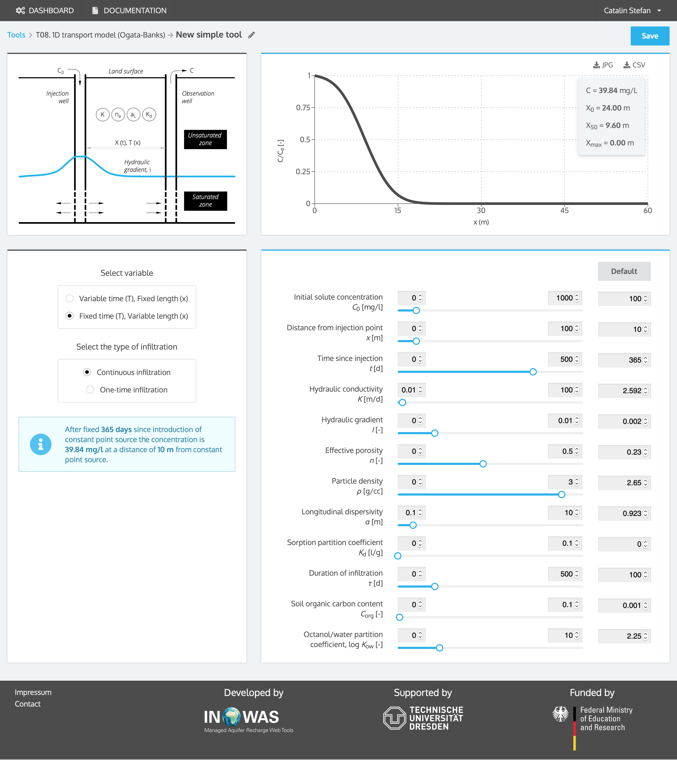
Infiltrated water containing Chlorid with a concentration of 100 mg/l enters an aquifer after passing the vadose zone with the following properties: Hydraulic conductivity K = 3.0 x 10⁻⁵ m/s; Hydraulic gradient I (dh/dl) = 0.002; Effective porosity ne = 0.23 >>> Resulting down gradient average fluid velocity vx = 2.6 x 10⁻⁷ m/s; Dispersion coefficient DL = 2.4 x 10⁻⁷ m2/s. Under assumption of no retardation the concentration of Chlorid in 1 year at a distance of 10 m from the point where the contaminated water entered the aquifer is 39.24 mg/l.
References
- Alvarez, P.J., Illman, W.A., 2005. Bioremediation and Natural Attenuation: Process Fundamentals and Mathematical Models. John Wiley & Sons.
- Bear, J., 1972. Dynamics of Fluids inPorous Media, Elsevier, New York.
- Gillham, R.W., Cherry, J.A., Barker, J.F., 1984. Groundwater Contamination. National Academies.
- Hölting, B., Coldewey, W.G., 2013. Hydrogeologie: Einführung in die Allgemeine und Angewandte Hydrogeologie. Springer-Verlag.
- Karickhoff, S.W., Brown, D.S., Scott, T.A., 1979. Sorption kinetics of hydrophobic pollutants in natural sediments. Water Resources 231–248.
- Ogata, A., Banks, R.B., 1961. A solution of the differential equation of longitudinal dispersion in porous media (US Geological Survey Professional Paper No. 411-A), Fluid Movement in Earth Materials. United States Government, Washington.
- Olshausen, H.-G., 2013. VDI-Lexikon Bauingenieurwesen. Springer-Verlag.
- Runkel, R.L., 1996. Solution of the advection-dispersion equation: Continuous load of finite duration. ResearchGate 122, 830–832.
- Sangster, J., 1989. Octanol‐Water Partition Coefficients of Simple Organic Compounds. Journal of Physical and Chemical Reference Data 18, 1111–1229. doi:10.1063/1.555833