The tool contains analytical equations that can be used to analyse or predict the location of the interface between sea water and fresh water in a groundwater system.
With the help of the Ghyben-Herzberg relation, the location of the interface between fresh and saltwater can be approximated under static hydraulic conditions (T09_a). The Glover equation provides also an indication of the shape and extent of the interface (T09_b). Upconing as a function of well pumping (T09_c) can be approximated by the equations developed by Schmork and Mercado, 1969 and Dagan and Bear, 1968. Critical well discharge (T09_d) can be calculated by the analytical equation of Strack, 1976. The effects of sea level rise on the migration of saltwater inland can be estimated using Werner and Simmons, 2009 (T09_e) when the coast can be assumed as a vertical cliff or Chesneaux, 2015 (T09_f) if the coast is inclined.
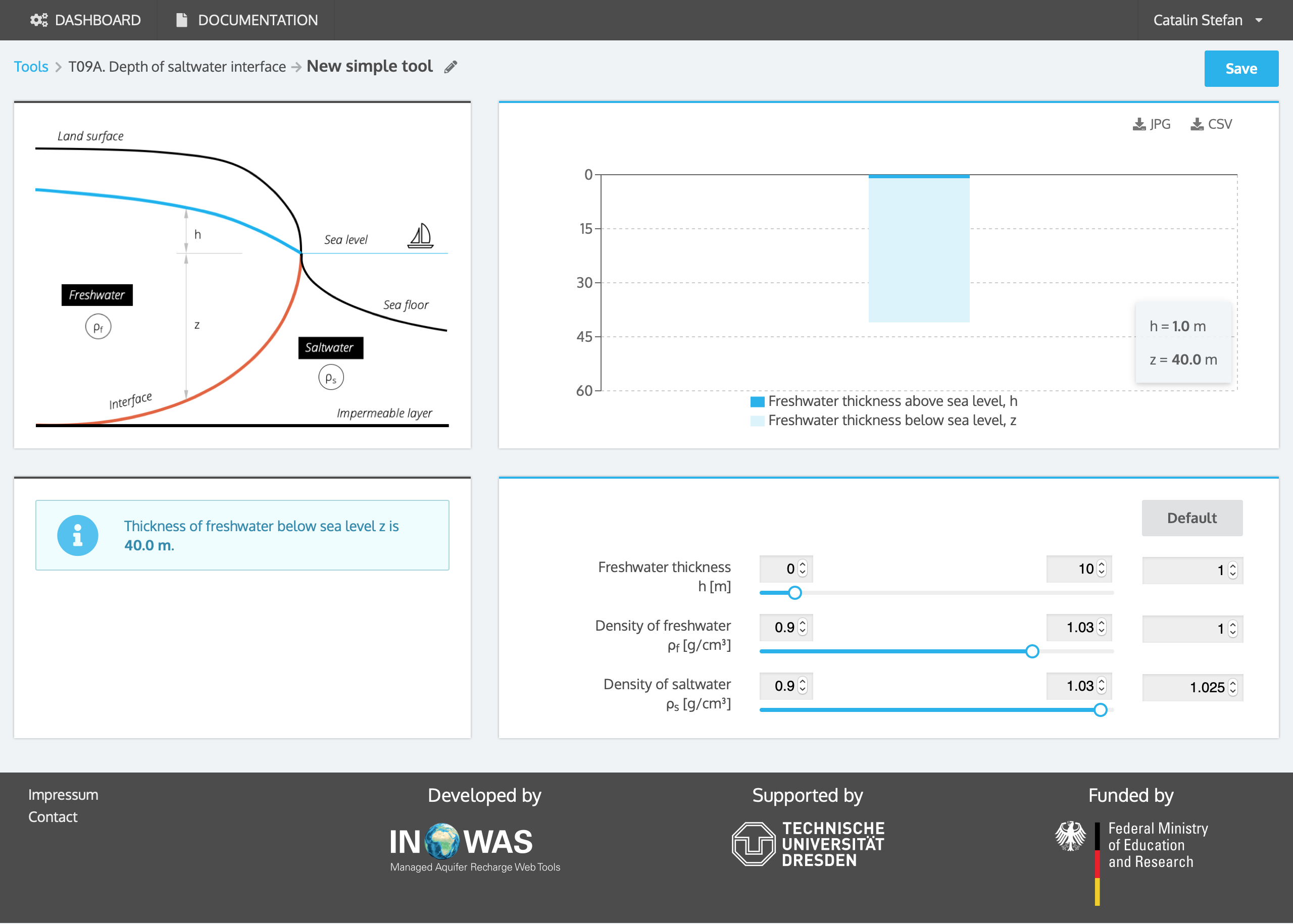
a. Depth of saltwater interface (Ghyben-Herzberg relation)
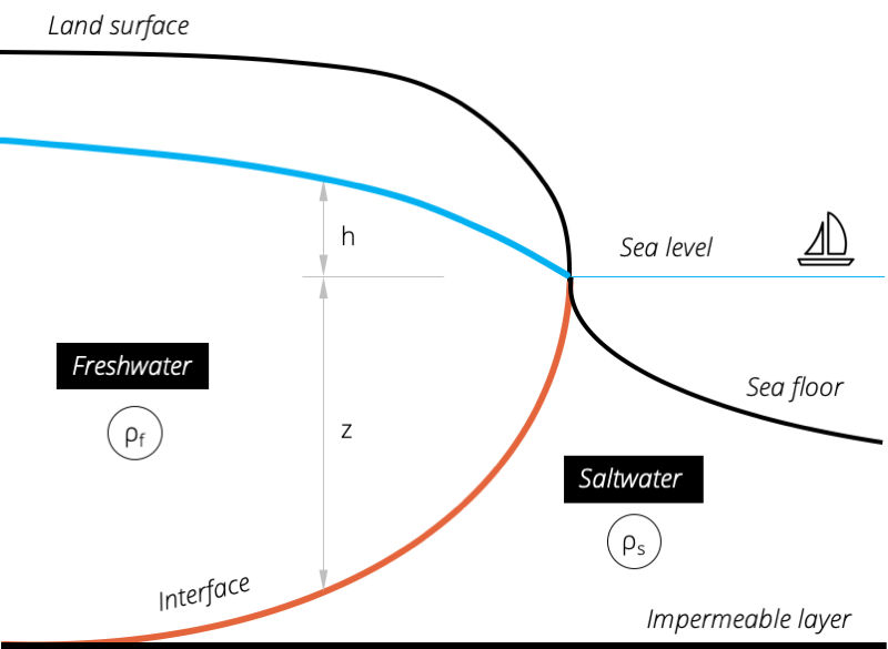
Figure 1. Schematic overview of the freshwater-saltwater interface in a coastal aquifer.
Under static hydraulic conditions, the interface between an area of fresh water and an area of sea water may be approximated by the difference in densities of fresh water and sea water.
| z=\frac{\rho_{f}}{(\rho_{s}-\rho_{f})}h_{f} | (eq. 1) |
with
| z | = thickness of freshwater below sea level [L] |
| h | = thickness of freshwater above sea level [L] |
| \rho_{f} | = density of freshwater [M/L³] |
| \rho_{s} | = density of saltwater [M/L³] |
Example
A groundwater well near the coast has not been pumped for years. Now, the total thickness of freshwater that might be available for development at the well site needs to be approximated. As a first estimate, the Ghyben-Herzberg equation is used. The elevation of the water table in the unpumped well is 10 m above sea level. Therefore, the estimated thickness of the fresh water zone underneath the sea water is 400 m and the total thickness of freshwater is 410 m (after Barlow, 2003).
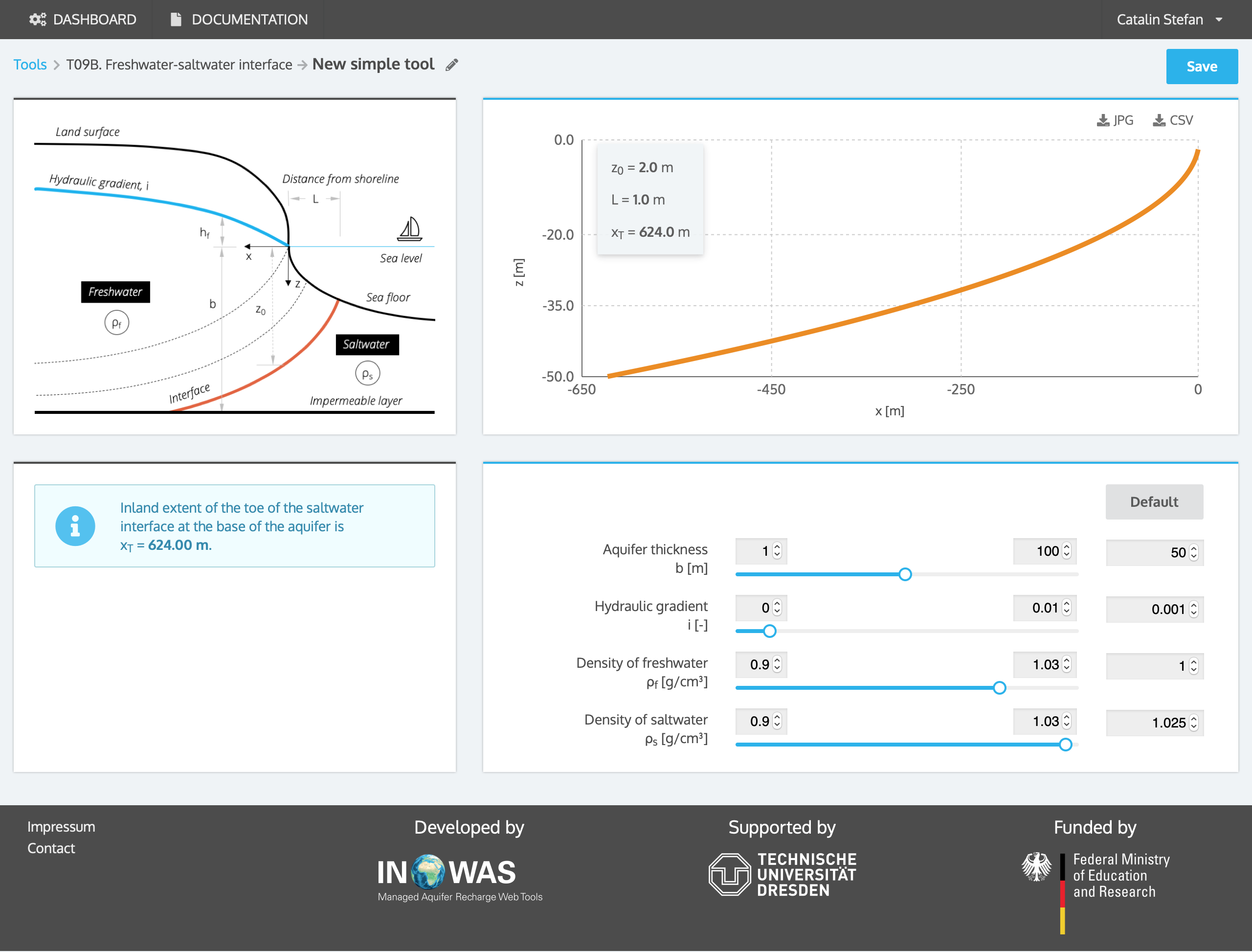
b. Freshwater-saltwater interface (Glover equation)
Glover’s equation takes into account the fresh water gradient to approximate the interface between an area of fresh water and an area of sea water and provides some indication of the shape and extent of the interface. In contrast to the Ghyben-Herzberg relation, freshwater discharges into the sea along an area rather than along a line.
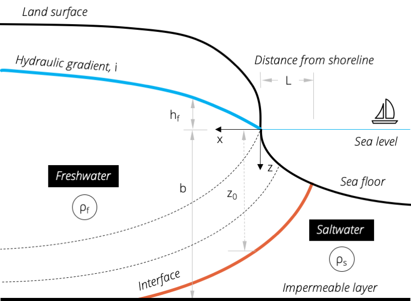
Figure 2. Shape and extent of the freshwater-saltwater interface in a coastal aquifer which can be calculated by the Glover equation.
| z^{2}=\frac{2qx\rho_{f}}{K(\rho_{s}-\rho_{f})}+\left[\frac{q\rho_{f}}{K(\rho_{s}-\rho_{f})}\right]^{2} | (eq. 2) |
where
| q | = freshwater outflow rate per unit length of coast line [L²/T] |
| K | = hydraulic conductivity [L/T] |
| x,z | = coordinate distances from shoreline [L] |
| \rho_{f} | = density of freshwater [M/L³] |
| \rho_{s} | = density of saltwater [M/L³] |
With the help of Darcy´s law, the equation can be rewritten as:
| z(x)=\sqrt{\frac{2ibx}{(\rho_{s}-\rho_{f})}+\left[\frac{ib\rho_{f}}{(\rho_{s}-\rho_{f})}\right]^{2}} | (eq. 3) |
where
| i | = hydraulic gradient [L/L] |
| b | = aquifer thickness [L] |
The shape of the fresh water table h_{f}( is defined as:
| h_{f}(x)=\sqrt{\frac{2ibx\rho_{f}}{(\rho_{s}-\rho_{f})}} | (eq. 4) |
The width of zone L, where freshwater flows into the sea (z=0) can be calculated as:
| L=\frac{ibx\rho_{f}}{2(\rho_{s}-\rho_{f})} | (eq. 5) |
The depth of the freshwater-saltwater interface beneath the shoreline (x=0) can be calculated using the following equation:
| z_{0}=\frac{ib\rho_{f}}{(\rho_{s}-\rho_{f})} | (eq. 6) |
Example
The location of the seawater-freshwater interface is approximated with the help of the Glover equation in a coastal aquifer where no pumping occurs. The hydraulic gradient is estimated to be 0.001. The aquifer thickness is 50 m. The depth of the interface beneath the shoreline is 2 m and the width of the zone where freshwater flows into the ocean is around 1 m.
c. Upconing
Upconing of the saltwater interface can occur when the aquifer head is lowered by pumping from wells. Schmork and Mercado, 1969 and Dagan and Bear, 1968 equations calculate upconing and the maximum well pumping rate at a new equilibrium caused by pumping. The pumping well is considered as a point.
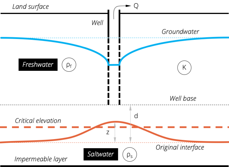
Figure 3. Upconing of the freshwater-saltwater interface by well pumping.
The maximum upconing, which happens directly underneath the pumping well, can be calculated as:
| z(0)=\frac{Q}{2\pi dK\varDelta\rho} | (eq. 7) |
As a guidance, Dagan and Bear (1969) propose that the interface will stay stable if the upconed height z does not exceed the critical elevation, which is defined as one-third of d (Callander et al., 2011). On that basis, the permitted pumping rate should not exceed:
| Q_{max}\leq\frac{0.6\pi d^{2}K}{\varDelta\rho} | (eq. 8) |
where \Delta\rho=\frac{\rho_{s}-\rho_{f}}{\rho_{f}} and
| z | = new equilibrium elevation (distance between the upconed and original interface) [L] |
| Q | = pumping rate [L³/T] |
| d | = pre-pumping distance from base of well to interface [L] |
| K | = hydraulic conductivity [L/T] |
To calculate the upconing at any distance from the well x, the following equation can be used (under steady state conditions t\rightarrow\infty)(Bear, 1999):
| z(x)=\left(\frac{1}{\sqrt{\frac{x^{2}}{d^{2}}+1}}-\frac{1}{\sqrt{\frac{x^{2}}{d^{2}}+\left(1+\frac{\varDelta\rho Kt}{nd(2+\varDelta\rho)}\right){}^{2}}}\right)\frac{Q}{2K\pi d\varDelta\rho} | (eq. 9) |
where
| n | = porosity [-] |
| t | = time [T] |
| x | = distance from well [L] |
Example
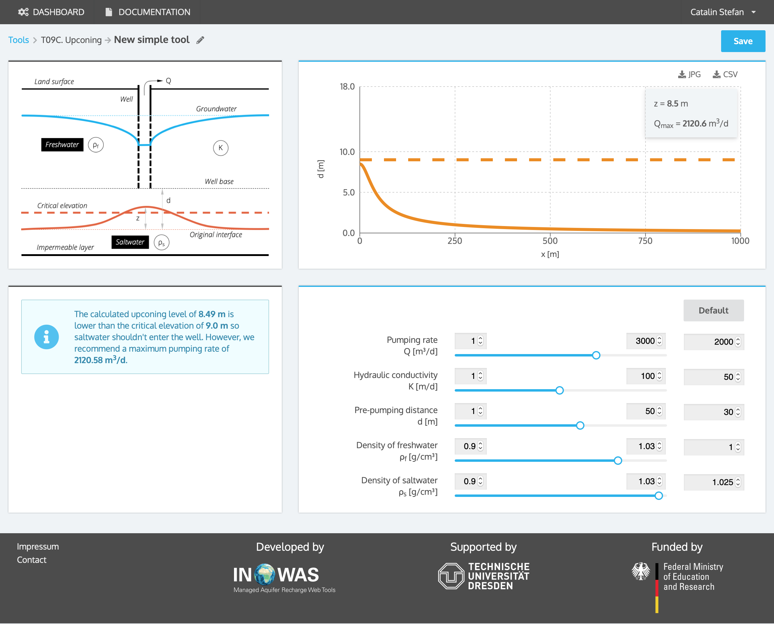
The pumping rate of a well in a coastal aquifer should be increased to 1000 m³/d and concerns exist, that saltwater which lies underneath the well, might intrude. Therefore, the upconing of the saltwater interface needs to be calculated. The aquifer has a hydraulic conductivity K of 50 m/d and the pre-pumping distance from the base of the well to the interface d is 30 m. The resulting saltwater upconing z is 4.2 m. The critical upconing elevation, which should not be exceeded, is 9.0 m and the corresponding critical well pumping rate is 2121 m³/d. Therefore, the pumping rate can be increased to the suggested amount without a high possibility of saltwater intrusion.
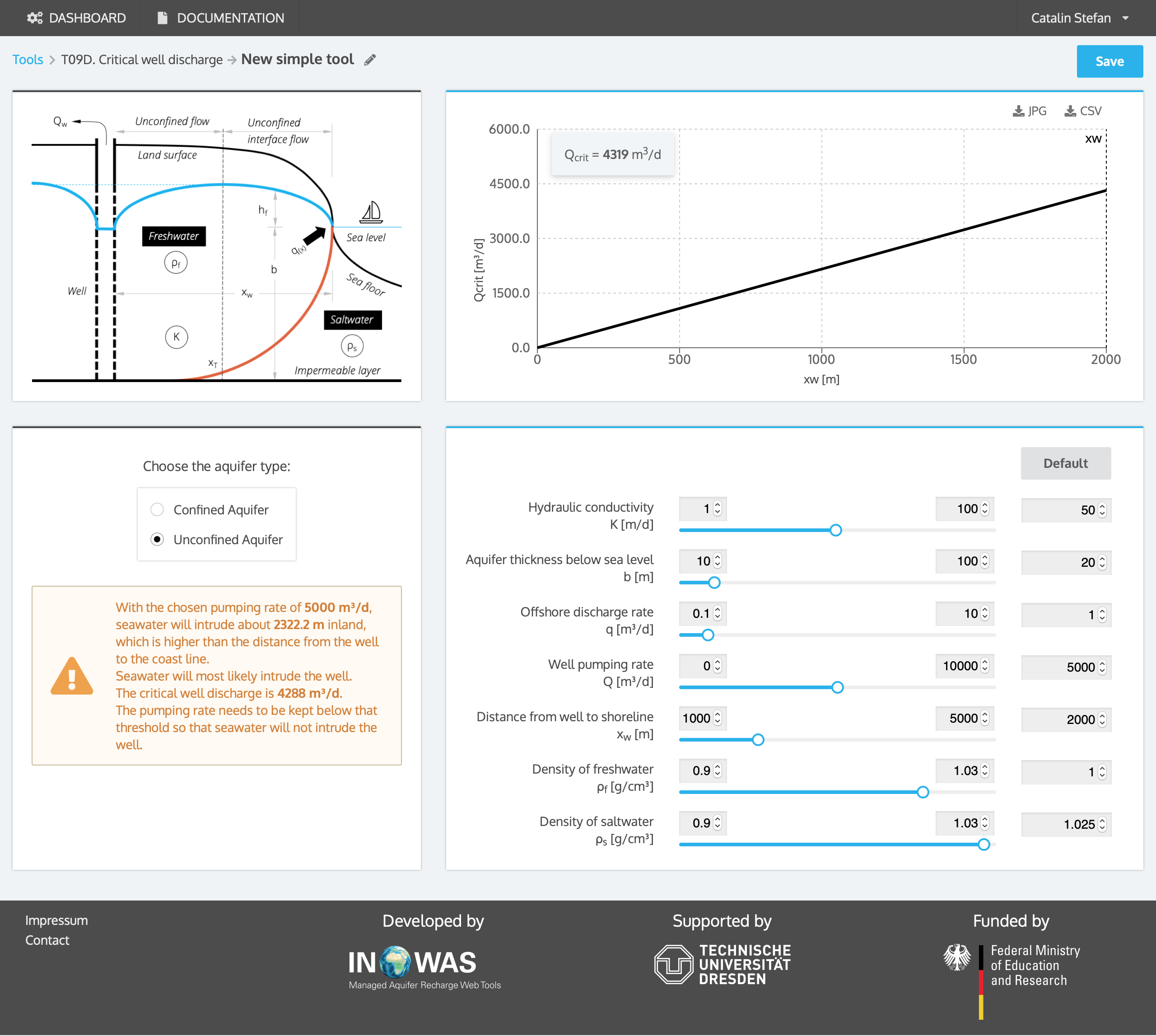
d. Critical well discharge
Strack (1976) introduced the concept of a critical abstraction rate which, if exceeded, creates an unstable situation where sea water will move inland to the well.
a)
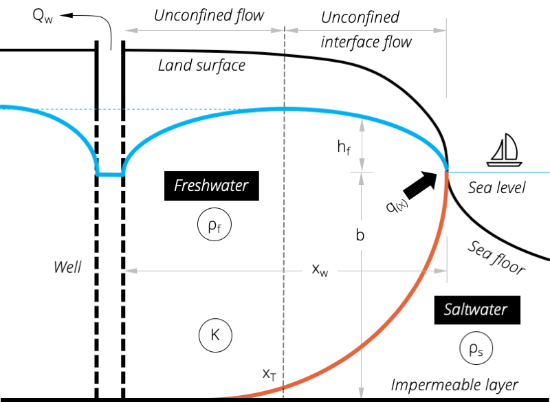
b)
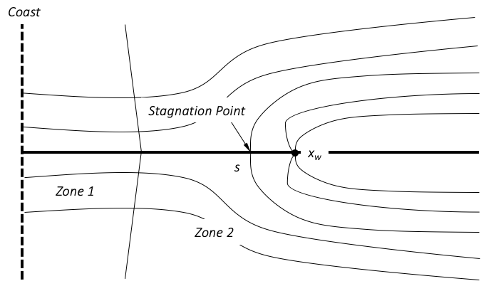
Figure 4. Pumping well in a coastal aquifer: a) cross-sectional view and b) plan view with Zone 1 referring to unconfined interface flow and Zone 2 to unconfined flow.
The equation to determine the position of the toe under steady conditions is given as followed (Callander, 2011):
| \frac{1}{2}\left(1+\varDelta\rho\right)\frac{z_{0}^{2}}{\varDelta\rho^{2}}=\frac{q}{K}x+\frac{Q_{W}}{4\pi K}ln\left[\frac{(x-x_{W})^{2}+y^{2}}{(x+x_{W})^{2}+y^{2}}\right] | (eq. 10) |
where \Delta\rho=\frac{\rho_{s}-\rho_{f}}{\rho_{f}}
| b | = depth to base of aquifer below mean sea level [L] |
| q | = fresh water flow per unit length of shoreline (assumed uniform) [L²/T] |
| Q_{W} | = constant pumping rate of the well superimposed on q [L³/T] |
| K | = hydraulic conductivity of the aquifer [L/T] |
| x_{W} | = distance between the well and the shoreline [L] |
| (x,y) | = x-y coordinates of the toe of the interface |
On the coastal side of the pumping well exists a stagnation point (x_{s}, y_{s}) which marks the divide between groundwater drawn towards the pumping well and groundwater flow towards the coast:
| x_{s}=x_{W}\left[1-\frac{Q_{W}}{{\pi}q_{out}x_{W}}\right];\quad y_{s}=0 | (eq. 11) |
When the toe of the interface passes through the stagnation point, the critical point of instability for the saltwater interface occurs and the saline water can move directly towards the well. The equations that define the critical pumping rate causing saline water to pass the stagnation point are:
| \lambda=\left(\frac{Kb^{2}}{qx_{W}}\right)\left(\frac{1+\varDelta\rho}{\varDelta\rho^{2}}\right) for unconfined aquifers or | (eq. 12a) |
| \lambda=\left(\frac{Kz_{0}^{2}}{qx_{W}\varDelta\rho}\right) for confined aquifers. | (eq. 12b) |
By using the value of \lambda calculated by equation (12a) and (12b) the following equation can be solved for \mu :
| \lambda=2\sqrt{\left(1-\frac{\mu}{\pi}\right)}+\frac{\mu}{\pi}ln\left[\frac{1-\sqrt{\left(1-\frac{\mu}{\pi}\right)}}{1+\sqrt{\left(1-\frac{\mu}{\pi}\right)}}\right] | (eq. 13) |
The critical well pumping rate Q_{crit} can then be calculated using \mu from equation (13):
| Q_{crit}=\mu qx_{W} | (eq. 14) |
The analytical solution is only valid for steady state in homogeneous isotropic aquifers where there is a hydraulic connection between the fresh water aquifer and the sea.
Example
The pumping rate Qw in a well which is screened along the total thickness of an unconfined coastal aquifer should be increased to 5000 m³/d. Concerns exist, that saltwater will intrude and reach the pumping well. The total thickness of the aquifer b is 20 m, the hydraulic conductivity K is 50 m/d and the fresh water flow q is 1 m³/d. The pumping well is located 2000 m from the coast line. With the help of the equation developed by Strack, 1978, the toe of the saltwater-freshwater interface under the assumed pumping rate Qw can be calculated. The toe of the saltwater-freshwater interface will intrude approximately 2322 m inland, which is higher than the distance of the well from the coastline. Therefore, saltwater will contaminate the well if it is pumped with the suggested rate of 5000 m³/d. The pumping rate should be less than the critical well discharge Q_{crit} which can also be calculated by the equation developed by Strack, 1978. The critical well discharge is 4286 m³/d which will keep the saltwater-freshwater interface stay stable and no saltwater will intrude the well.
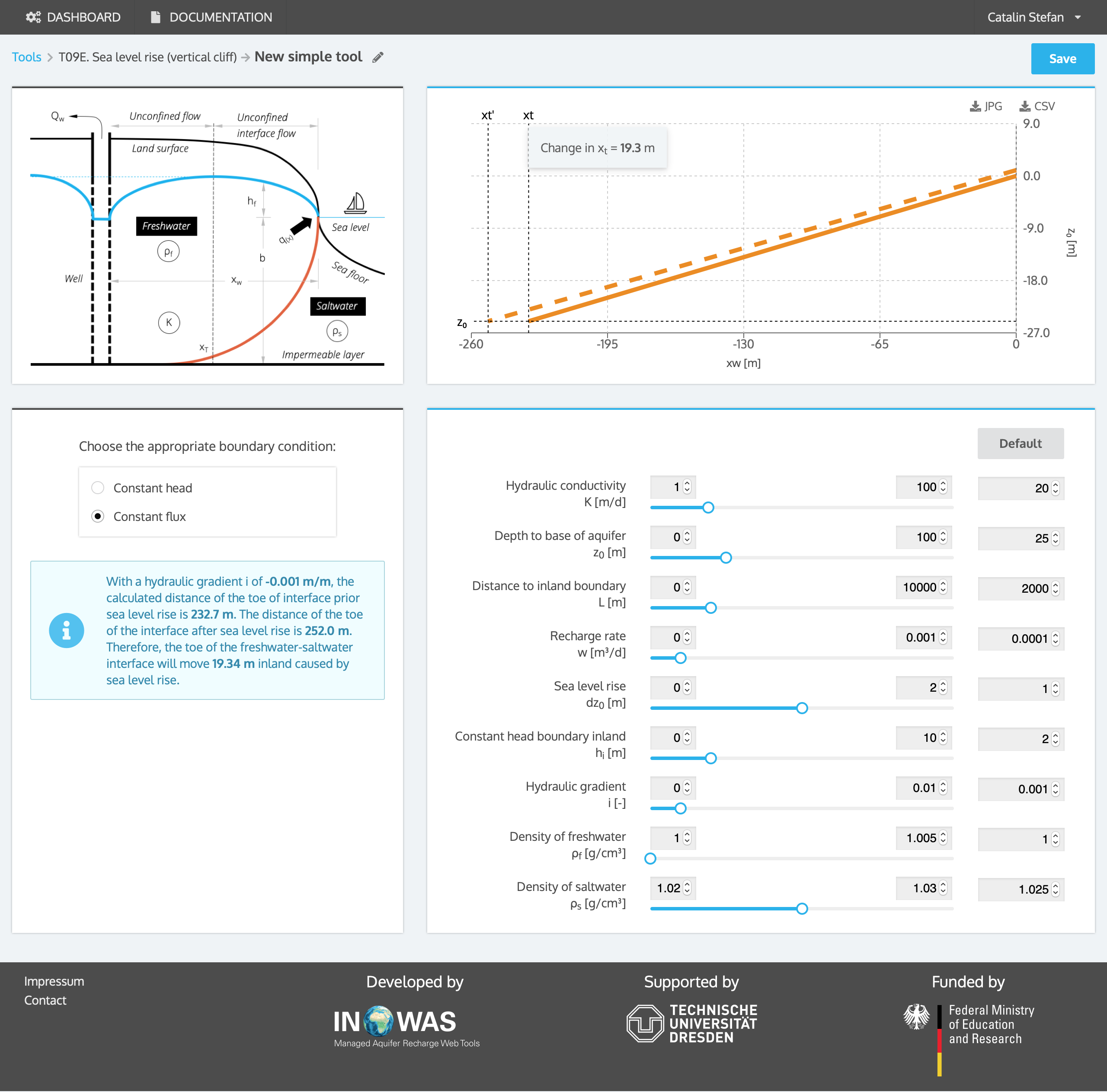
e. Sea level rise (vertical cliff)
Contains equations presented by Werner and Simmons, 2009 on the effects of sea level rise on sea water intrusion. These equations can be used to estimate the inland migration of the toe of the fresh water sea water interface in response to sea level rise, where there is a constant head boundary inland or constant flux inland. In the case of constant head, groundwater throughflow and the offshore discharge will decrease in response to sea level rise. If there is no constant head present, the water table height will increase in response to sea level rise (constant flux).
- flux-controlled system: groundwater discharge is persistent despite changes in sea level (hydraulic gradient at inland boundary is constant);
- head-controlled system: surface features or groundwater abstractions maintain the head condition in the aquifer despite sea level change (hydraulic head at inland boundary is constant).
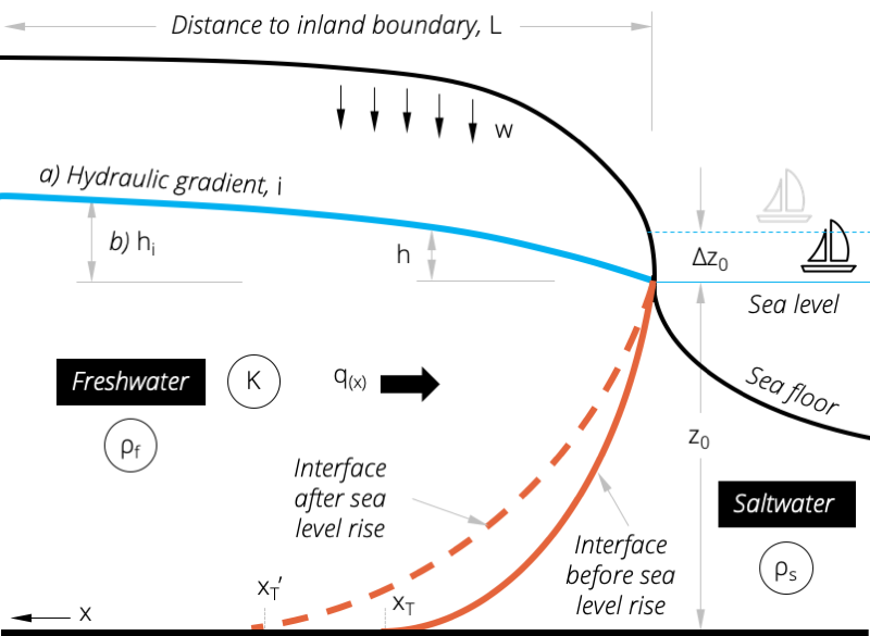
Figure 5. Inland migration of the toe of the freshwater-saltwater interface caused by sea level rise.
To define the position of the toe of the interface (x_{T}), three equations need to be solved iteratively. First, the fresh water head h in the zone of the saltwater interface (0<x<x_{T}) is defined as:
| h=\sqrt{\frac{2q_{0}x-Wx^{2}}{K(1+\varDelta\rho)}} | (eq. 15) |
where
| x | = distance inland from the position of the coast line [L] |
| x_{T} | = inland extent of the toe of the saltwater interface at the base of the aquifer [L] |
| q_{0} | = discharge of fresh groundwater into the sea per unit length of coastline [L²/T] |
| W | = surface recharge to the aquifer [L/T] |
| K | = hydraulic conductivity of the aquifer [L/T] |
The toe of the saltwater-freshwater interface intersects the base of the aquifer at an inland distance x_{T} which can be calculated as:
| x_{T}=\frac{q_{0}}{W}-\sqrt{\frac{q_{0}}{W}-\frac{K(1+\varDelta\rho)z_{0}^{2}}{W\varDelta\rho^{2}}} | (eq. 16) |
where
| z_{0} | = depth below sea level to the base of the aquifer [L]. As the reference point for
this parameter is mean sea level, it increases as sea level rises. |
Additionally, the solution must also fit the definition of fresh water head h on the inland side of the toe of the saltwater-freshwater interface (x>x_{T}):
| h=\sqrt{\frac{2}{K}(x-x_{T})\left(q_{0}-\frac{W}{2}\left(x+x_{T}\right)\right)+(h_{T}+z_{0})^{2}} | (eq. 17) |
The previous three equations (15), (16) and (17) can only be solved iteratively to define how the position of the toe of the saltwater interface could change as a result of sea level rise, if the following constraints are met:
Equations (15) – (17) do not define a realistic inland position of the fresh water head but create a water table mound at a distance that can be defined as follows:
x_{m}=\frac{q_{0}}{W} at which point q_{0}(x_{m})=0.
As the area of interest is between the coast and the inland distance x_{T}, the parameters used in the equations (15) -(17) must always ensure that x_{m}>x_{T}. This is achieved by ensuring that q>q_{min} where
q_{min}=\sqrt{\frac{WK(1+\varDelta\rho)z_{0}^{2}}{\varDelta\rho^{2}}}
General assumptions inherent are that the aquifer is isotropic and homogeneous, a sharp saltwater-freshwater interface exists, steady state conditions and constant recharge applies.
Example 1: constant head
In a coastal aquifer, the impact of 1 m sea level rise on the inland migration of seawater is evaluated. The aquifer has a hydraulic conductivity K of 20 m/d and an aquifer thickness z0 of 25 m. The recharge rate W is 0.0001 m/d. The constant head hi at the inland boundary, which is 2000 m from the coast, is 2 m. Iterating the equations developed by Werner and Simmons, 2009, the off-shore discharge rate pre-sea level rise was calculated to be 0.54 m²/d and the toe of the interface is located 304 m inland. After a sea level rise of 1 m, the off-shore discharge rate decreases to 0.29 m²/d and the toe of the interface is 686 m inland. Therefore, the toe of the freshwater-seawater interface will move 381 m inland because of the assumed sea level rise.

Example 2: constant flux
In a coastal aquifer, the impact of 1 m sea level rise on the inland migration of seawater is evaluated. The aquifer has a hydraulic conductivity K of 20 m/d and an aquifer thickness z0 of 25 m. The recharge rate W is 0.0001 m/d. A constant flux at the inland boundary 2000 m inland, is assumed. At the inland boundary, the hydraulic gradient i is 0.001 m/m which equals an aquifer throughflow rate of 0.5 m²/d. The calculated distance of the toe of interface prior sea level rise is 232.7 m, the distance after sea level rise is 252.0 m. Therefore, the toe of the freshwater-saltwater interface will move 19.3 m inland because of the assumed sea level rise.
F. Sea level rise (inclined coast)
With the help of the analytical solution by Chesnaux (2015) the inland toe migration within coastal aquifers caused by sea level rise can be approximated. In contrast to the solution by Werner and Simmons (2009), the equation considers a low inclination of the sea shore and hence progressions of the sea boundary inland due to sea level rise (Figure 6).
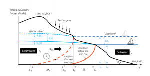
Figure 6. Inland migration of the freshwater-saltwater interface due to sea level rise considering the low inclination of the sea shore (after Chesnaux, 2015).
According to Morgan and Werner (2016), the solution developed by Chesnaux (2015) is only valid for a fixed-location, no-flow boundary (fixed-flux) in a continental unconfined aquifer. Hence, the geological limit of the aquifer is used as the inland boundary and other cases such as a head-dependent boundary (e.g. through pumping, evapotranspiration, rivers, drains) are not considered. To assess the impact of sea level rise in fixed-head aquifers, the solution by Werner and Simmons (2009) (assuming a vertical cliff) or the more generalizable solution by Ataie-Ashtiani et al. (2013) can be used.
The initial position of the toe of the freshwater saltwater interface can be calculated using the following equation:
| x_{T}=\sqrt{L_{0}^{2}-\left(\frac{z_{0}}{\alpha\beta}\right)^{2}} | (eq. 18) |
With \alpha=\sqrt{\frac{w\varDelta\rho}{K(\rho_{f}+\Delta\rho)}} and \beta=\frac{\rho_{f}}{\Delta\rho}
and where z0 is initial depth below sea level to the aquifer basement (impermeable bottom) [L], W is surface recharge of the aquifer [LT-1], K is hydraulic conductivity of the aquifer [LT-1], L0 is initial width of the aquifer [L], ρf is freshwater density [ML-3], ρs is sea water density [ML-3], Δρ [ML-3] is the density difference between fresh and saltwater and can be calculated as .
The fluctuation of the height of the aquifer at any position x when sea level changes can be calculated using the following equation:
| I(x)=\Delta z_{0}+\sqrt{\frac{-\alpha^{2}\Delta z_{0}}{tan\theta}*\left(2L_{0}-\frac{\Delta z_{0}}{tan\theta}\right)+h_{0}(x)^{2}}-h_{0}(x) | (eq. 19) |
With where x [L] is the inland distance from the position of the coast line, θ is the slope of the coastal aquifer [°], h0(x) is the initial water table at position x in the aquifer [L] and Δz0 is sea level change [L].
The change in position of the sea water toe due to sea level changes can be calculated as follows:
| \Delta x_{T}=\sqrt{\left(L_{0}-\frac{\Delta z_{0}}{tan\theta}\right)^{2}-\left(\frac{z_{0}+\Delta z_{0}}{\alpha\beta}\right)^{2}}-\sqrt{L_{0}^{2}-\left(\frac{z_{0}}{\alpha\beta}\right)^{2}} | (eq. 20) |
Example
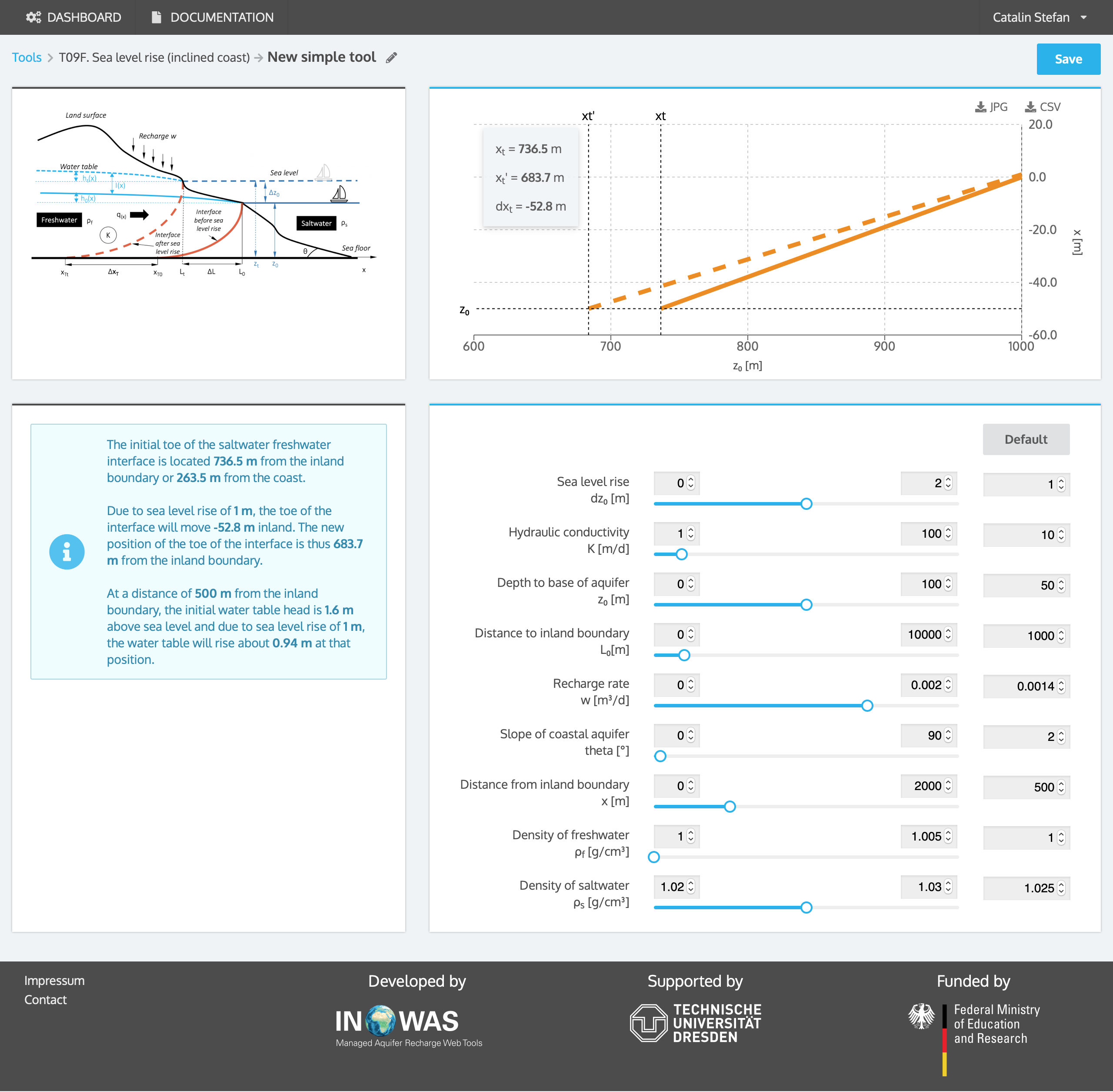
In a coastal aquifer, the impact of 1 m sea level rise on the inland migration of seawater is evaluated. The aquifer has a hydraulic conductivity K of 10 m/d and an aquifer thickness z0 of 50 m. The recharge rate W is 1.4*10-3 m/d. The initial aquifer width L (distance to inland boundary) is 1000 m. The slope of the coastal aquifer is 2°. The initial toe of the saltwater freshwater interface is located 736.5 m from the inland boundary or 263.5 m from the coast. Due to sea level rise, the toe of the interface will move 52.8 m inland. The new position of the toe of the interface is thus 683.7 m from the inland boundary. At a distance of 500 m to the coast, the initial water table head is 1.6 m above sea level and due to sea level rise the water table will rise about 1.001 m at that position.
References
-
- Ataie-Ashtiani, B., Werner, A.D., Simmons, C.T., Morgan, L.K., Lu, C., 2013. How important is the impact of land-surface inundation on seawater intrusion caused by sea-level rise? Hydrogeology Journal 21, 1673–1677. https://doi.org/10.1007/s10040-013-1021-0
- Barlow, P.M., 2003. Ground Water in Freshwater-Saltwater Environments of the Atlantic Coast, USGS Circular 1262.
- Bear, J. (Ed.), 1999. Seawater intrusion in coastal aquifers: concepts, methods and practices, Theory and applications of transport in porous media. Kluwer, Dordrecht.
- Callander, P., Lough, H., Steffens, C., 2011. New Zealand Guidelines for the Monitoring and Management of Sea Water Intrusion Risks on Groundwater. Pattle Delamore Partners LTD, New Zealand.
- Chesnaux, R., 2015. Closed-form analytical solutions for assessing the consequences of sea-level rise on groundwater resources in sloping coastal aquifers. Hydrogeology Journal 23, 1399–1413. https://doi.org/10.1007/s10040-015-1276-8
- Dagan, G., Bear, J., 1968. Solving The Problem Of Local Interface Upconing In A Coastal Aquifer By The Method Of Small Perturbations. Journal of Hydraulic Research 6, 15–44. doi: 10.1080/00221686809500218
- Glass, J., Jain, R., Junghanns, R., Sallwey, J., Fichtner, T., Stefan, C., 2018. Web-based tool compilation of analytical equations for groundwater management applications. Environmental Modelling & Software 108, 1–7. https://doi.org/10.1016/j.envsoft.2018.07.008.
- Morgan, L.K., Werner, A.D., 2016. Comment on “Closed-form analytical solutions for assessing the consequences of sea-level rise on groundwater resources in sloping coastal aquifers”: paper published in Hydrogeology Journal (2015) 23:1399–1413, by R. Chesnaux. Hydrogeology Journal 24, 1325–1328. https://doi.org/10.1007/s10040-016-1398-7
- Schmork, S., Mercado, A., 1969. Upconing of Fresh Water-Sea Water Interface Below Pumping Wells, Field Study. Water Resources Research 5, 1290–1311. doi: 10.1029/WR005i006p01290
- Strack, O.D.L., 1976. A single-potential solution for regional interface problems in coastal aquifers. Water Resources Research 12, 1165–1174. doi: 10.1029/WR012i006p01165
- Verruijt, A., 1968. A note on the Ghyben-Herzenberg formula. International Association of Scientific Hydrology. Bulletin 13, 43–46. doi: 10.1080/02626666809493624
- Werner, A.D., Simmons, C.T., 2009. Impact of Sea-Level Rise on Sea Water Intrusion in Coastal Aquifers. Ground Water 47, 197–204. doi: 10.1111/j.1745-6584.2008.00535.x