Travel times and capture zones are essential parameters used to delineate groundwater and wellhead protection zones and to design ground water remediation systems. This tool is based on the works of (Chapuis and Chesnaux, 2006) and (Chesnaux et al., 2005) and depicts travel time calculations in an unconfined aquifer under selected boundary conditions.
The solution can be applied to steady-state, saturated flow systems with a flow that is considered horizontal and one dimensional according to the Dupuit approximation (Haitjema, 1995; Kirkham, 1967). The unconfined aquifer is recharged by constant surface infiltration and discharges to a fixed-head boundary condition. Bottom condition is an impervious layer. The system is bound by constant head boundary conditions, no flow boundaries or pumping wells. The soil is assumed to be homogenous and groundwater heads and velocities are assumed to not vary with depth. Surface infiltration is included as uniform annual rate. Please note, that only positive net recharge can be considered.
The tool on hand presents four different options of boundary conditions that bound the aquifer. For users that are unsure about the conditions of their regional flow system a mechanism is included to help decide which set of boundaries apply (option 4: T13_d).
The tool can be applied for the following boundary conditions:
- Aquifer system with one no-flow boundary and one fixed head boundary condition and constant groundwater recharge (T13_a)
- Aquifer system with two fixed head boundary conditions, a flow divide within the system and constant groundwater recharge (T13_b)
- Aquifer system with two fixed head boundary conditions, a flow divide outside of the system and constant groundwater recharge (T13_c)
- Aquifer system with two fixed head boundary conditions, constant groundwater recharge but user is not sure whether the flow divide lies within the system (T13_d)
- Aquifer system with one pumping well at constant rate, no groundwater recharge (T13_e)
The first four options are based on the work of Chesnaux et al. (2005). The last option has been developed by Chapuis and Chesnaux (2006).
a. Aquifer system with a no-flow boundary and fixed head boundary condition and constant groundwater recharge
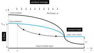
The left-hand boundary is impermeable (flow divide), and flow discharges through the right-hand fixed-head boundary. The travel time is calculated between the two arbitrary points: xi(the departure point at the water table) and x. This flow system is used for developing the general analytical solution. Systems for the other options (option 2-4) are eventually transformed into this system.
Table 1. Notation of input parameters needed for the calculation of transient time
| W | = uniform, annual average rate of infiltration | LT-1 |
| K | = hydraulic conductivity of the aquifer | LT-1 |
| ne | = effective porosity | – |
| L‘ | = length of the aquifer | L |
| hL‘ | = downstream fixed head boundary | L |
| xi | = initial position | L |
| x | = downgradient arrival location at which the transit time will be determined ( xi< x < L’ ) | L |
The transient time t(T)between xiand x is then calculated with the analytical equation:
| (eq. 1) |
where
| (eq. 2) |
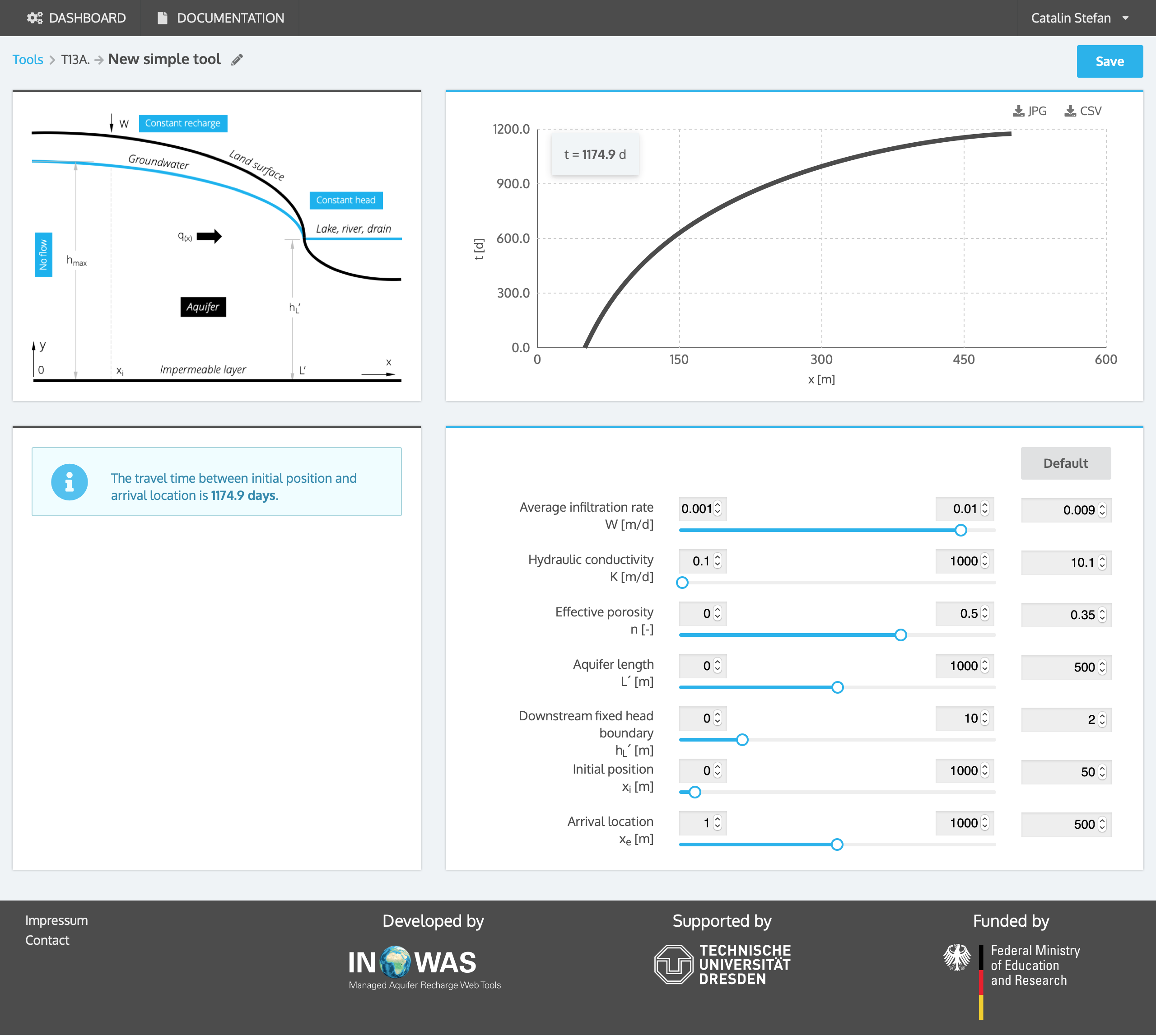
Example
The travel time is calculated between the two arbitrary points: xi= 50 m (the departure point at the water table) and 500 m for an aquifer of 500 m length. The left-hand boundary is impermeable (flow divide) and flow discharges through the right-hand fixed-head boundary with a fixed head boundary of hL’=2 m. The aquifer is characterized by an effective porosity of 0.35 and a hydraulic conductivity of 10.1 m/d. The aquifer is recharge by a uniform, annual average rate of infiltration of 0.009 m/d. The travel time between both points is calculated to be 1175 days.
b. Aquifer system with two fixed head boundary conditions, a flow divide within the system and constant groundwater recharge
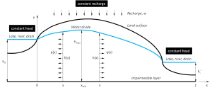
The system is bound by two fixed-head boundary conditions and contains a flow divide between these two boundaries.
Table 2. Notation of input parameters needed for the calculation of transient time
| L | = length of the aquifer | L |
| K | = hydraulic conductivity of the aquifer | LT-1 |
| h0 | = upstream head at x = 0 with h0 > hL | L |
| hL | = downstream head at x = L | L |
| W | = uniform, annual average rate of infiltration | LT-1 |
| ne | = effective porosity | – |
| xi | = initial position | L |
| x | = downgradient arrival location at which the transit time will be determined ( xi < x < L’ ) | L |
The tool first calculates xWD[L] which is the position of the water divide based on equation 3 (Bear, 1972):
| (eq. 3) |
The location of the water divide depends on the relative magnitude of the boundary heads h0and hLas well as the recharge and hydraulic conductivity. From Equation 3, we can deduce that the condition of applies to this set of boundaries.The regional flow system is then separated into two subdomains on either side of the water divide and the user can chose which subdomain he wants to use for calculation.
If the right subdomain is considered:
L’ =L – xWD and hL’= hL
If the left subdomain is considered:
L = xWD and hL’ = h0
Calculation of travel time then proceeds based on equation 1 and 2.
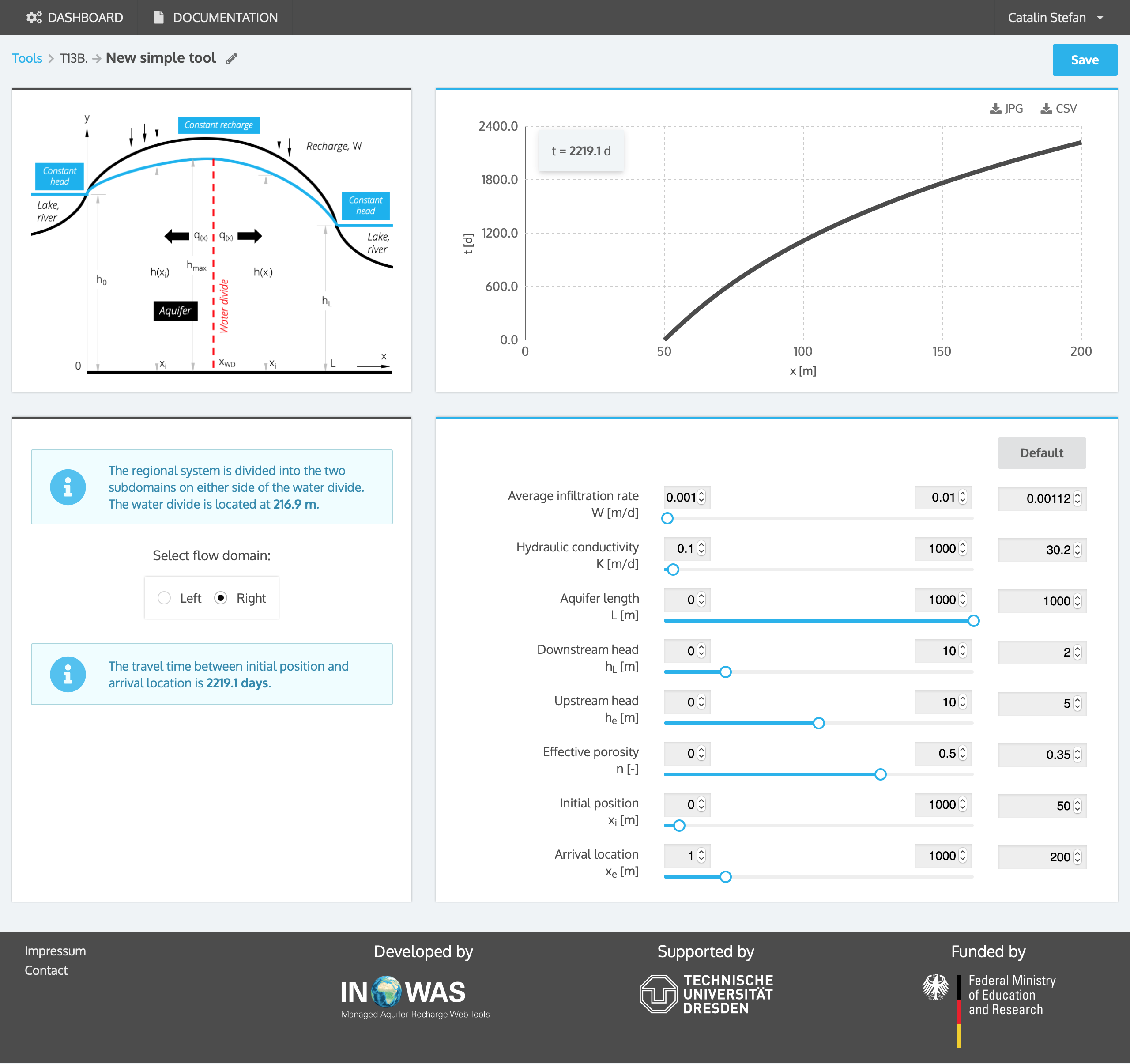
Example
An aquifer of 1000 m length is bound between two fixed head boundaries with h0=5 m and hL=2 m. The aquifer is recharge by a uniform, annual average rate of infiltration of 0.00112 m/d and has an effective porosity of 0.35 as well as a hydraulic conductivity of 30.2 m/d. The flow divide lies within the system and is calculated to be at position xWD=216.9 m. Choosing the right side of the flow domain, the aquifer length is set to 783.1 m. The travel time between xi=50 m and x=700 m is the calculated to be 3960 days. If the left side of the flow domain is chosen the aquifer length is set to 216.9 m and the travel time between xi=50 m and x=200 m is calculated to be 2219 days.
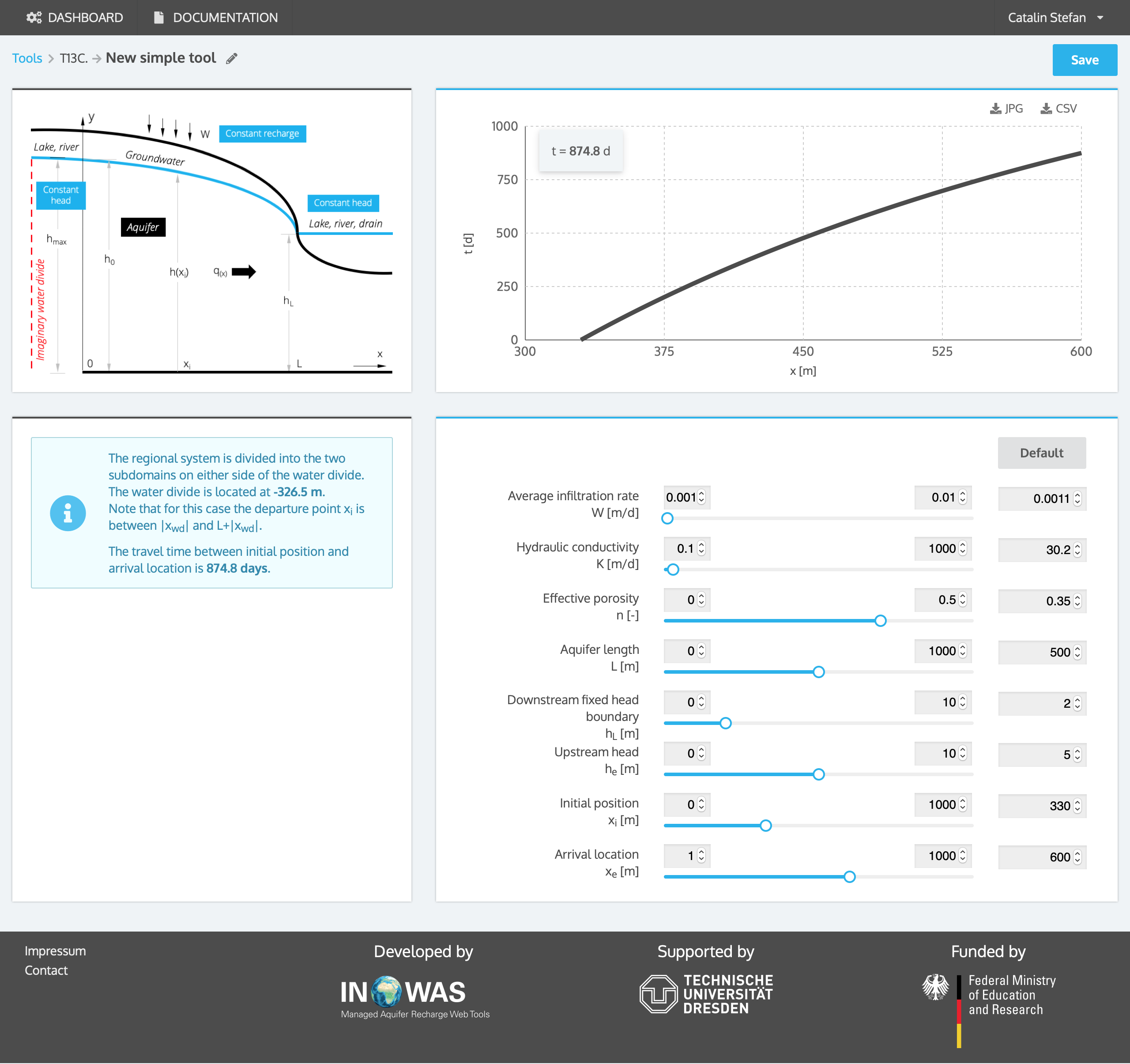
c. Aquifer system with two fixed head boundary conditions, a flow divide outside of the system and constant groundwater recharge
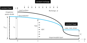
The system is bound by two fixed-head boundary conditions and contains a flow divide outside of these two boundaries. Flow is unidirectional between the constant head boundaries. The flow divide is imaginary and is located upgradient of the constant head boundary at x = 0.
Input parameters for this option are the same as shown in table 2.
The tool first calculates the position of the water divide based on equation 3. The location of the water divide depends on the relative magnitude of the boundary heads h0and hLas well as the recharge and hydraulic conductivity. From Equation 3, we can deduce that the condition of applies to this set of boundaries.
For the case of an imaginary water divide:
L’ = L + abs(xWD) and hL’= hL
Note that for this case the departure point xiis between |xWD| and L’!
Calculation of travel time then proceeds based on equation 1 and 2.
Example
An aquifer of 500 m length is bound between two fixed head boundaries with h0=5 m and hL=2 m. The aquifer is recharged by a uniform, annual average rate of infiltration of 0.0011 m/d and has an effective porosity of 0.35 as well as a hydraulic conductivity of 30.2 m/d. The flow divide lies outside of the system and is calculated to be at position xWD=-326.5 m. The flow system is thus extended and the aquifer length is set to be 826.5 m. The travel time is calculated between xi=330 m and x=600 m. Note that the starting point should be greater than 326.5 m in order to lie within the original aquifer system. The travel time between both points is calculated to be 875 days.
d. Aquifer system with two fixed head boundary conditions, constant groundwater recharge but user is not sure whether the flow divide lies within the system
If the user is not certain whether the flow divide lies within the system, the tool provides an option to calculate the water divide based on the input parameters in table 2 and equation 3. If xWD > 0 the flow divide lies within the flow system and the tool will proceed with option 2. If xWD < 0 the flow divide lies outside of the system and the tool will proceed option 3.
After setting the input parameters, the tool displays in the left hand panel the appropriate option for further calculations. By clicking on the left panel, the user is then send to the subsequent sub-tool 13_b or 13_c.
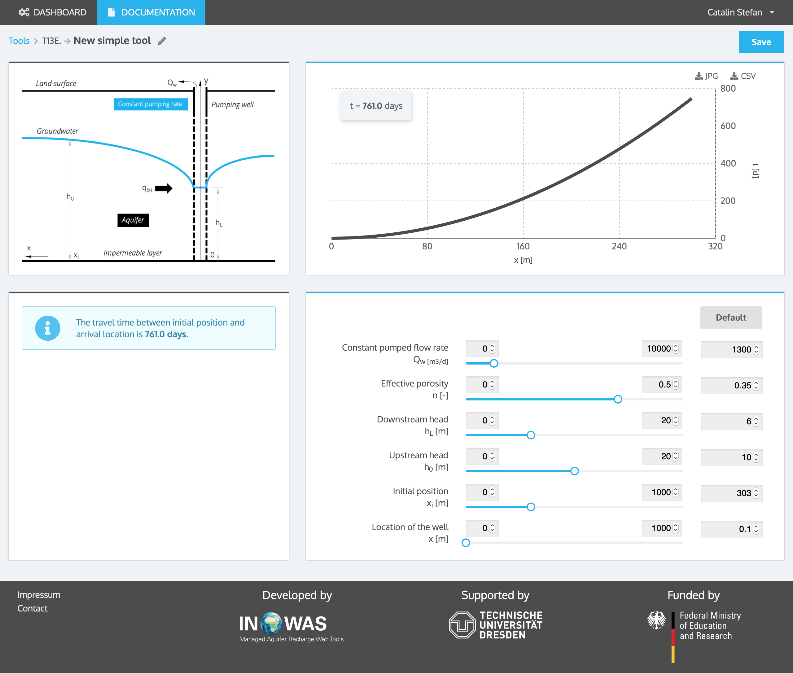
e. Aquifer system with one pumping well at constant rate, no groundwater recharge
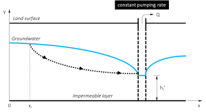
This option is based on the work of (Chapuis and Chesnaux, 2006) and is used to calculate the travel time to a pumping well in horizontal unconfined aquifer with negligible recharge. A closed-form solution is available; this tool presents the simplified analytical equation.
Table 3. Notation of input parameters needed for the calculation of transient time
| QW | = constant pumped flow rate | L³T-1 |
| ne | = effective porosity | – |
| h0 | = upstream head at initial position | L |
| hL | = downstream head (at well location) | L |
| xi | = initial position | L |
| x | = location of the well | L |
Since it is recommended in practice to operate the pumping well with a ratio hL/hR≥ 0.5 (with hRbeing the upstream head at the maximum radius of influence of the well), and considering the characteristics of the function h(x), haveis very close to h0, the largest head at the starting point. For quick evaluations, it is proposed here to estimate haveas equal to 95% of h0 (the largest value at the farthest distance xi) plus 5% of hL(the smallest value at the shortest distance x), thus eq. 4 is can be used as a simplified equation for calculation the travel time through the aquifer to a pumping well.
| (eq. 4) |
Example
Travel time between xi=303 m and the outer boundary of a well at x=0.1 m is calculated. The pumping rate of the well is 1300 m³/d and the aquifer has an effective porosity of 0.35. The upstream head at the initial position is 10 m and the downstream head at well location is 6 m. The travel time towards the well is calculated to be 2.08 years.
References
- Bear, J., 1972. Dynamics of fluids in porous media. Dover Publications Inc., New York.
- Chapuis, R.P., Chesnaux, R., 2006. Travel Time to a Well Pumping an Unconfined Aquifer without Recharge. Ground Water 44, 600–603. doi:10.1111/j.1745-6584.2006.00141.x
- Chesnaux, R., Molson, J.W., Chapuis, R.P., 2005. An analytical solution for ground water transit time through unconfined aquifers. Ground Water 43, 511–517. doi:10.1111/j.1745-6584.2005.0056.x
- Haitjema, H.M., 1995. Analytic Element Modeling of Groundwater Flow. Academic Press, Bloomington, Indiana.
- Kirkham, D., 1967. Explanation of paradoxes in Dupuit-Forchheimer Seepage Theory. Water Resour. Res. 3, 609–622. doi:10.1029/WR003i002p00609