Subsurface travel time from the area of recharge to the point of abstraction during MAR is a critical parameter to ensure sufficient attenuation for hygienic parameters and other undesired substances. This tool helps to determine groundwater hydraulic residence time (HRT) using seasonal temperature fluctuations observed in recharge water and MAR recovery wells. This tool represents a proxy for quick, cost-effective and reliable control of travel time during aquifer passage.
This tool was developed within the frame of SMART-Control, a WaterJPI project. For further information please visit: www.smart-control.inowas.com.
The documentation of the tool is based on the SMART-Control Deliverable 4.1.
Time series of seasonal temperature measurements observed in surface water and abstraction wells can be fitted to sinusoidal functions. Peak values represented as local maxima and local minima and turning points from the fitted sinusoidal curves are used for the approximation of travel times between surface water and abstraction well. The calculated values are adjusted by a thermal retardation factor.
Theoretical background
The scientific background of the tool is rooted in the hypothesis that seasonal temperature variations in surface waters and abstraction wells can be used as potential tracers to estimate the groundwater hydraulic residence time during subsurface passage. At MAR sites, the groundwater temperature is directly influenced by seasonal temperature variations in the influent surface water. Under ideal conditions, these variations underlay a sinusoidal curve, with maximum values achieved in summer and lowest in winter. Under real conditions however, the approach needs to take into account also the retardation of heat transport in the subsurface due to multiple physical and site-specific factors. Thus, the real groundwater transport velocity is faster than the pore water velocity, leading to groundwater flowing faster than the temperature front propagation and the need of a correction factor accounting for this thermal retardation.
The mathematical concept of the tool consists in using a non-linear regression for fitting a sinusoidal curve to time series of temperature measurements taken at the points of recharge and extraction. To obtain plausible results it is necessary to select a full sine curve at both the inflow (surface water) and the outflow (groundwater), corresponding usually to a complete one-year cycle. After data selection the measured temperatures are fitted for each full sine period separately to the general sinusoidal form according to:
f(x)=y_{0}+A*\sin\left(\pi\frac{x-x_{c}}{w}\right)where:
y_{0} = vertical shift or off-set
A = amplitude
x_{c} = horizontal shift or phase shift
{w} = period
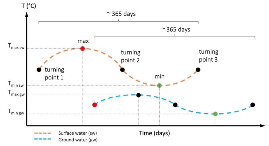
This non-linear fitting is an iterative process carried out until convergence is reached. The fitted sine curve is then used to identify the dates of the peak values (local minima and maxima) and turning points (Figure 1). The time difference of the extrema between basin (surface water) and well (groundwater) results in a time offset that corresponds to the groundwater hydraulic residence time. However, heat is transported not only by the flowing water (convective heat flow), but also by heat exchange through solids and fluids (conductive heat flow). The mutual heat exchange of groundwater with the surrounding aquifer material retains the heat signal compared to pure advective transport, resulting in attenuation and retardation of the temperature signal along the flow path. Calculated lag times between peak values and turning points in the basin and corresponding peak values in the groundwater need to be therefore corrected by a thermal retardation factor.
The tool is based on a previously developed algorithm in R language which is currently available on the GitHub repository at https://github.com/KWB-R/kwb.heatsine.
Preparation of data
The first step consists in uploading temperature measurement time series, one for the surface water that is infiltrated and one for the groundwater at the point of extraction. For this, the INOWAS tool “T10 Real-time monitoring” is used. In T10, sensors can be created, sensor data uploaded as well as time and value processing executed for data preparation. As the heat transport tool required a time series of about a year, the time series need to be cropped using the time processing function “cut”. If the time series uploaded contains data from several years, try to select the year that is most representative and for which the seasonal variations can be described best by a sinusoidal curve. For more details see “Deliverable 4.1“.
Calculation and results visualisation
To calculate the groundwater residence time using temperature time series uploaded in previous steps, open the tool T19 “Groundwater residence time” and create a new simulation. In the opening window, select the file with time series corresponding to surface water and groundwater temperature from the list of T10 instances. Note
that the list contains all public instances of T10, including those created by other users. After choosing the instance, select the observation point (“sensor”) for both inflow and outflow (Figure 2). In the example below, both time series have been prepared in T10 by selecting time range values between 23.04.2016 – 30.05.2017 for surface water and 19.06.2016 – 29.06.2017 (for groundwater), each interval representing approximately one year.
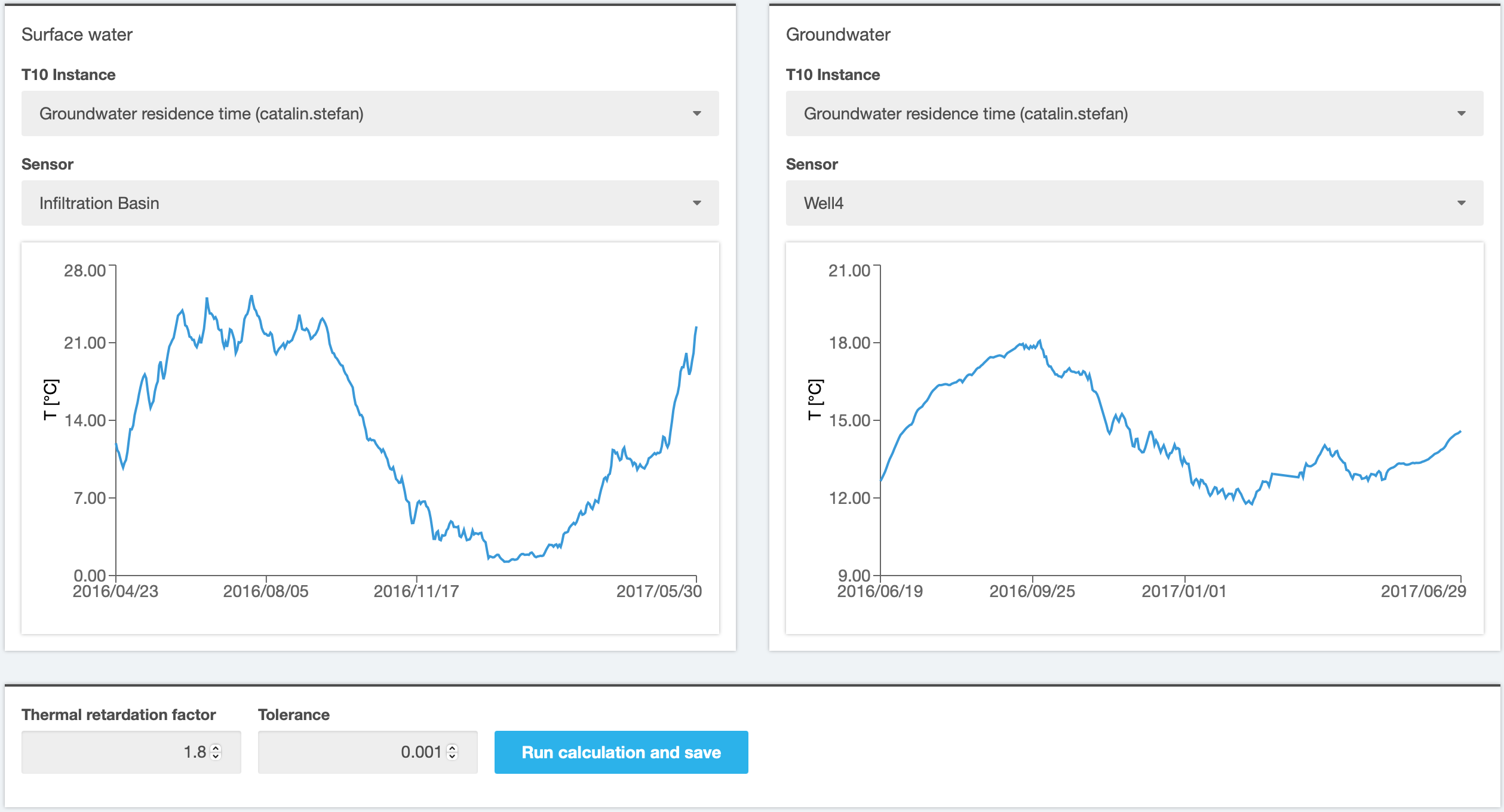
By default, a thermal retardation factor of 1.8 is considered, which corresponds to a sandy aquifer. The value can be edited, then the calculation can be started by clicking the button “Run calculation and save”.
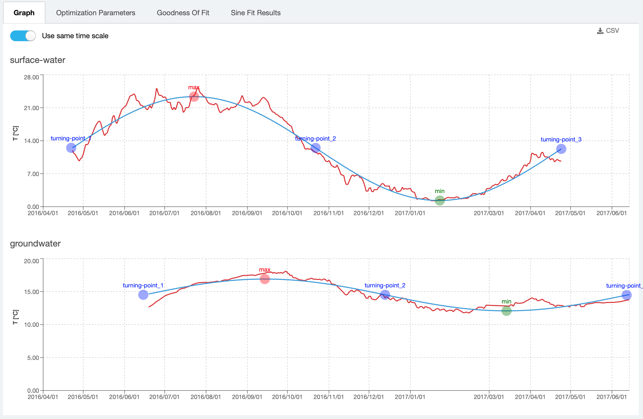
The results of the calculation are shown in Figure 3. The sine curve (blue line) is fitted to the temperature measurements (red line) and the max/min and observation points are displayed on the graphs. To facilitate visualisation and comparison, both graphs can be displayed using the same time scale (which emphasizes the time shift between temperature measurements in inflow/outflow) or by adjusting the time scale (in which case the curves are superimposed).
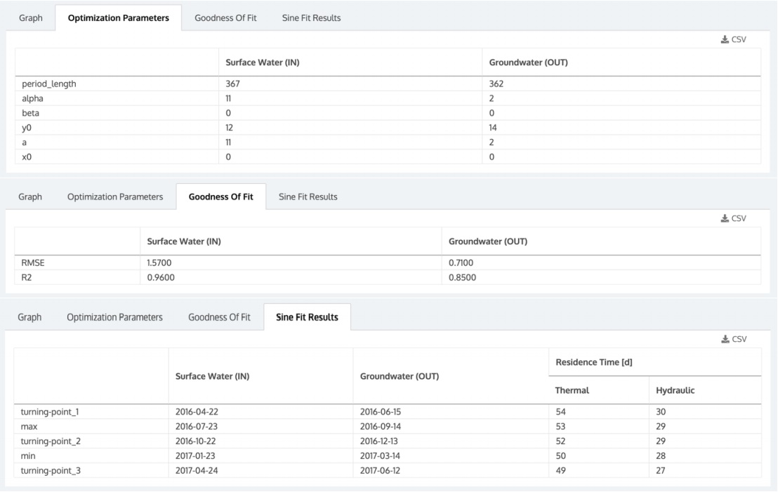
The other three tabs in the results section show the optimization parameters of the sinusoidal regression curve (see Eq. 1), the goodness of fit to the measured temperature data and, in the last tab, the times corresponding to the calculated max and min temperatures and the three turning points, as well as the calculated groundwater
residence time with and without consideration of the retardation factor (thermal / hydraulic) (Figure 4). Each result can be then downloaded as CSV file.